Probability Patterns and Chance

Name: Probability Patterns and Chance
Availability: InStock

An introductory course on probability, designed for beginners to understand patterns and chance through practical examples.

My workspace30 minFree to watch

What you’ll learn

01Introduction to Probability: Patterns and ChanceWelcome. This course is about recognizing patterns in chance and making better decisions when things are uncertain. Probability gives us a logical way to describe what we know and what we cannot know for sure. You already use these ideas every day: checking a weather forecast, estimating travel time, or weighing a business risk. In this training, we will build on that everyday reasoning. We work from the idea of uncertainty itself, then introduce the sample space, events, and the key concept of long‑run frequency. You will see how probabilistic thinking differs from assuming a single cause‑and‑effect chain, because it works with likelihood and evidence instead. There is no advanced math required, only concrete examples you can apply right away. By the end, you will sharpen how you communicate risk and use data to make informed choices under uncertainty. Let us start by asking a simple but powerful question: What does uncertainty really mean?stat.berkeley.edu link.springer.com stats.stackexchange.com+21 min
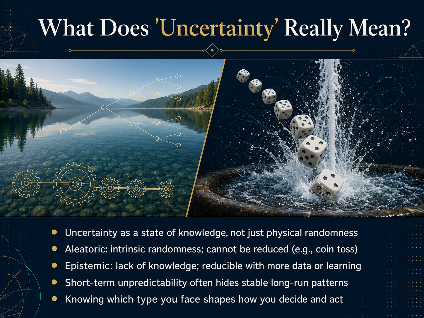
02What Does 'Uncertainty' Really Mean?Now, let's get more precise about the word 'uncertainty'. In the language of probability, it's not just one big, vague cloud. It's helpful to think of uncertainty as a state of knowledge, not just physical randomness. There are two key types you need to recognize. The first is aleatoric uncertainty. This is intrinsic randomness, the irreducible kind. Think of a fair coin toss. No matter how much data you collect, you can't predict the next flip with certainty. The variability is built into the system. The second is epistemic uncertainty. This comes from a lack of knowledge. It's what you feel when you don't know a fact that someone else does, like the exact temperature in the server room right now. This type is reducible. You can eliminate it by getting more data or learning. Here's why the distinction matters. The short-term unpredictability you see in a coin toss or a stock price often hides stable long-run patterns. Knowing whether you're facing aleatoric randomness or an epistemic knowledge gap directly shapes how you decide and act. Do you gather more information, or do you build a system that's robust to the noise? Recognizing that is the first practical step. With this framework in mind, we can now start mapping out what could happen. Let's move to the next slide on sample spaces.stat.berkeley.edu link.springer.com stats.stackexchange.com+22 min
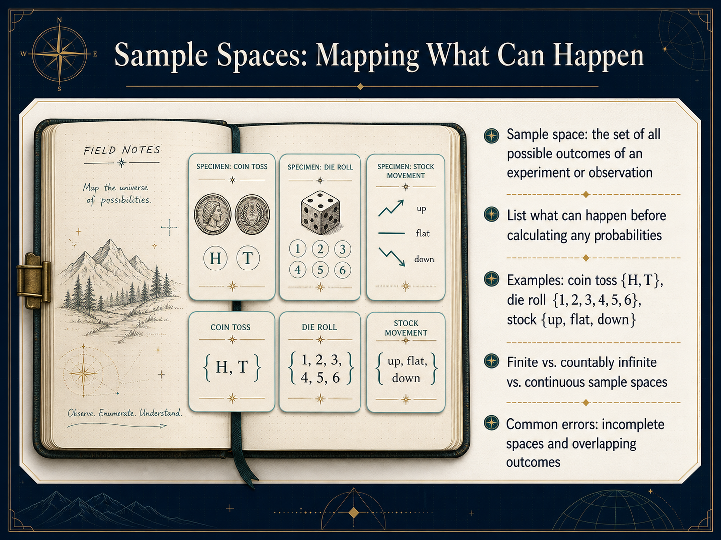
03Sample Spaces: Mapping What Can HappenNow let's talk about sample spaces. Think of a sample space as a map of everything that could possibly happen in a given situation. It's the full set of all possible outcomes, and our first job is simply to list them out before we start calculating anything. For a coin toss, the sample space is heads and tails. For rolling a standard die, it's the numbers one through six. In a work context, if you're looking at a daily stock movement, the sample space might simply be up, flat, or down. Sample spaces can be different sizes too. Some are finite, like a die roll. Others are countably infinite or even continuous, like measuring the exact temperature outside. The most common mistake at this stage is creating an incomplete space or having outcomes that overlap, which makes solid analysis impossible. So, the key habit is to pause and map out the full set of possibilities first. Next, we'll look at how to group these outcomes into events that actually matter for decision-making.blog.vistaslearning.com eecs70.org probability4datascience.com+22 min
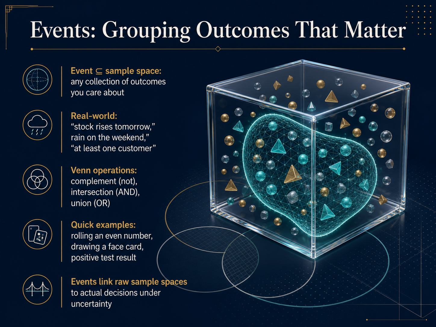
04Events: Grouping Outcomes That MatterNow let's focus in on events. An event is simply any collection of outcomes from your sample space that you care about for a particular decision. Think of it as a subset of the sample space. For example, the sample space for tomorrow's weather might include sunny, rainy, and cloudy. The event you care about is just rain. Other real-world events could be a stock price rising, having at least one customer call, or drawing a face card from a deck. We also use a few simple operations to combine events, just like with sets. The complement of an event means 'not' that event happening. Intersection means both events happen together, an 'and' situation. Union means at least one of the events happens, an 'or' situation. So, rolling an even number is an event made of the outcomes two, four, and six. A positive medical test result is an event that drives a decision. Events are the crucial link. They take the raw list of possibilities in the sample space and group them into the specific questions that actually guide what we do next. Now that we can group outcomes into meaningful events, let's explore how we assign numbers to them. Our next step is to define probability as a long-run relative frequency.blog.vistaslearning.com eecs70.org probability4datascience.com+22 min
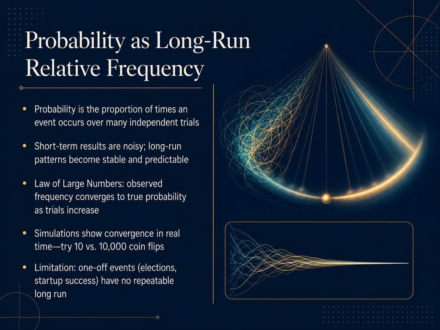
05Probability as Long-Run Relative FrequencyNow, let's make this idea of probability more precise. Think of probability as the long-run relative frequency of an event. That simply means the proportion of times something happens over many, many independent trials. In the short term, results are noisy—flip a coin ten times, and you might get seventy percent heads. That's completely normal. But if you keep flipping, the pattern stabilizes. After ten thousand flips, that percentage will hover very close to fifty percent. This stability is captured by the Law of Large Numbers, which tells us that as the number of trials increases, the observed frequency converges to the true probability. Simulations make this visible in real time, letting you compare ten flips against ten thousand. There is one crucial limitation to keep in mind though. This long-run thinking works for repeatable events like coin flips or insurance claims, but not for one-off events. Unique situations—like a specific election outcome or the success of a single startup—don't have a repeatable long run. Next, let's build from this foundation and explore the axioms and basic rules of probability.demonstrations.wolfram.com onlinemathlearning.com web-apps.thecoatlessprofessor.com+22 min
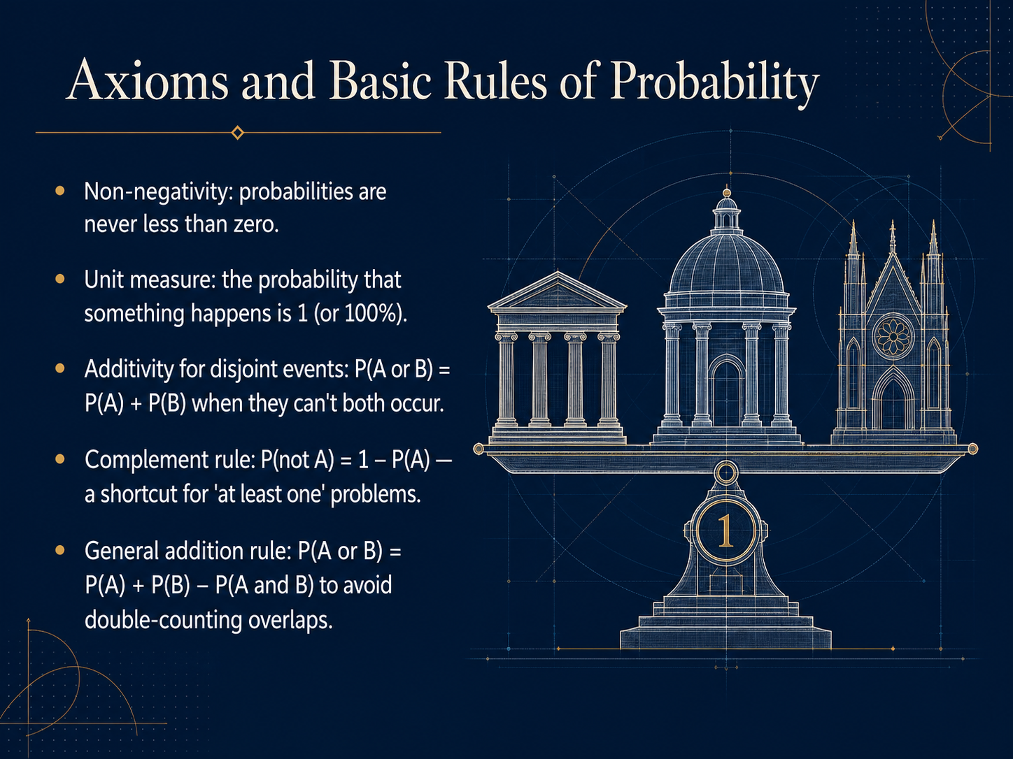
06Axioms and Basic Rules of ProbabilityNow, let's solidify our understanding with the fundamental building blocks: the axioms and basic rules of probability. These aren't just abstract math; they are simple, logical constraints that keep our reasoning about chance consistent and useful. First, probabilities are never negative. A negative chance doesn't make sense, so this rule, called non-negativity, gives us a floor. Second, the probability that something—anything—in our sample space happens is one, or one hundred percent. This is the unit measure, and it confirms that our list of possible outcomes is complete. Third, we have the additivity rule for mutually exclusive, or disjoint, events. If two outcomes cannot both occur, like flipping a heads or tails on a single coin toss, the probability of one or the other happening is simply the sum of their individual probabilities. A handy corollary is the complement rule: the probability of an event not happening is one minus the probability that it does. For instance, if a critical server has a five percent chance of failing this year, the probability it doesn't fail is ninety-five percent. This is a powerful shortcut for 'at least one' problems. Finally, when events do overlap, like the chance of rain or a traffic jam, we use the general addition rule. We add the individual probabilities but subtract the overlap once to avoid double-counting. These rules are our toolkit for navigating uncertainty. Next, we will explore how these rules apply when we move from frequency to subjective probability.blog.vistaslearning.com eecs70.org probability4datascience.com+22 min
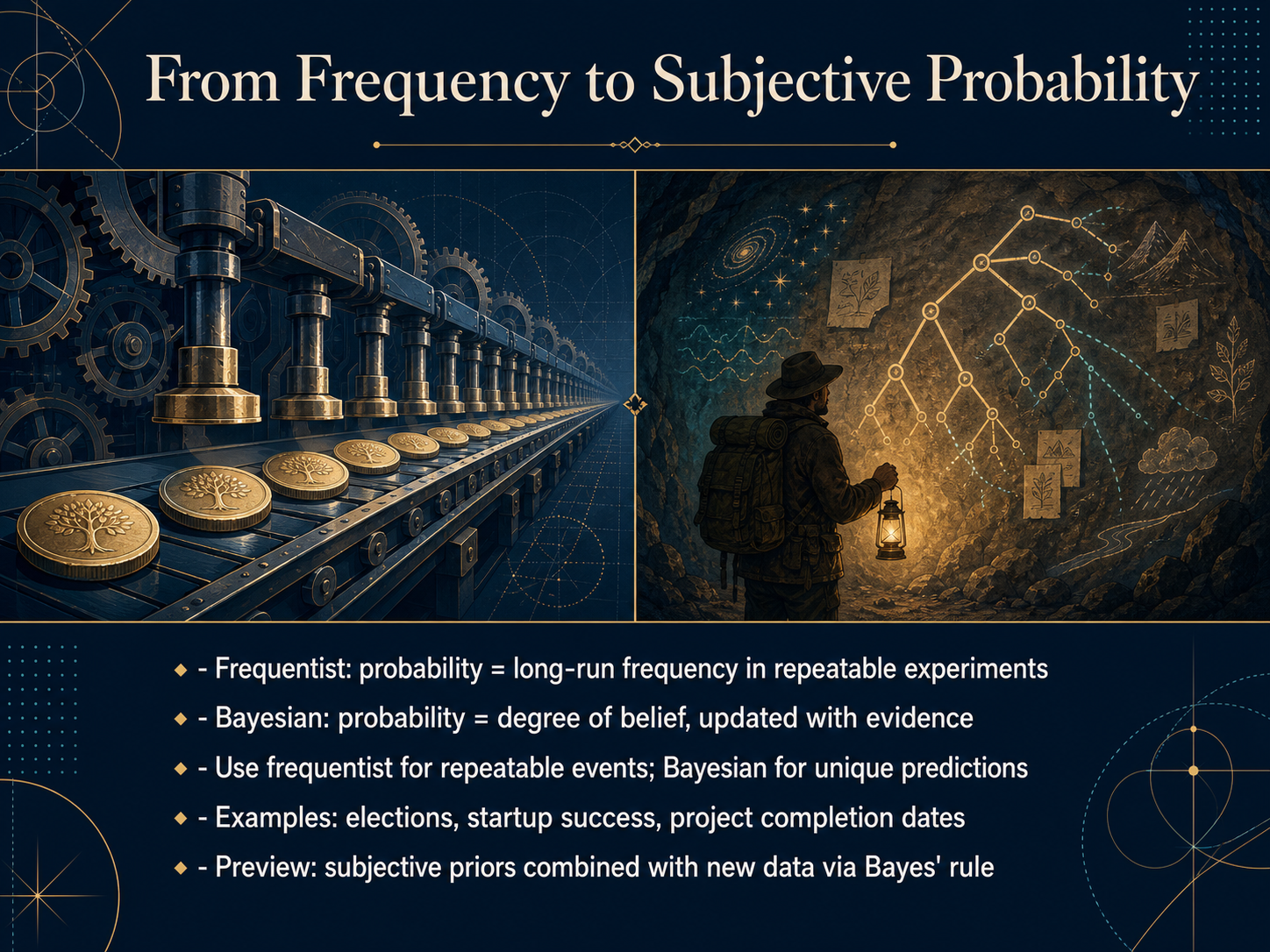
07From Frequency to Subjective ProbabilityNow we connect those core ideas to two main schools of thought. The frequentist view treats probability as a long-run frequency in repeatable experiments. Think of flipping a coin thousands of times, the probability of heads is the proportion you would see over the long haul. The Bayesian view treats probability as a degree of belief that gets updated as new evidence arrives. It is a measure of confidence, not just repetition. When should you use each? Frequentist thinking works well for clearly repeatable events. But for unique, one-time predictions, Bayesian thinking gives us a natural language. Imagine predicting an election outcome, the success of a startup, or whether a project will finish on time. You cannot re-run those events thousands of times. Up next, we will preview how Bayesians combine a subjective starting belief, called a prior, with fresh data, using Bayes' rule. But first, let's explore another fundamental pattern, what happens when chance is repeated many times. That brings us to the law of large numbers.statsig.com thedatacopywriter.substack.com bookdown.org+22 min
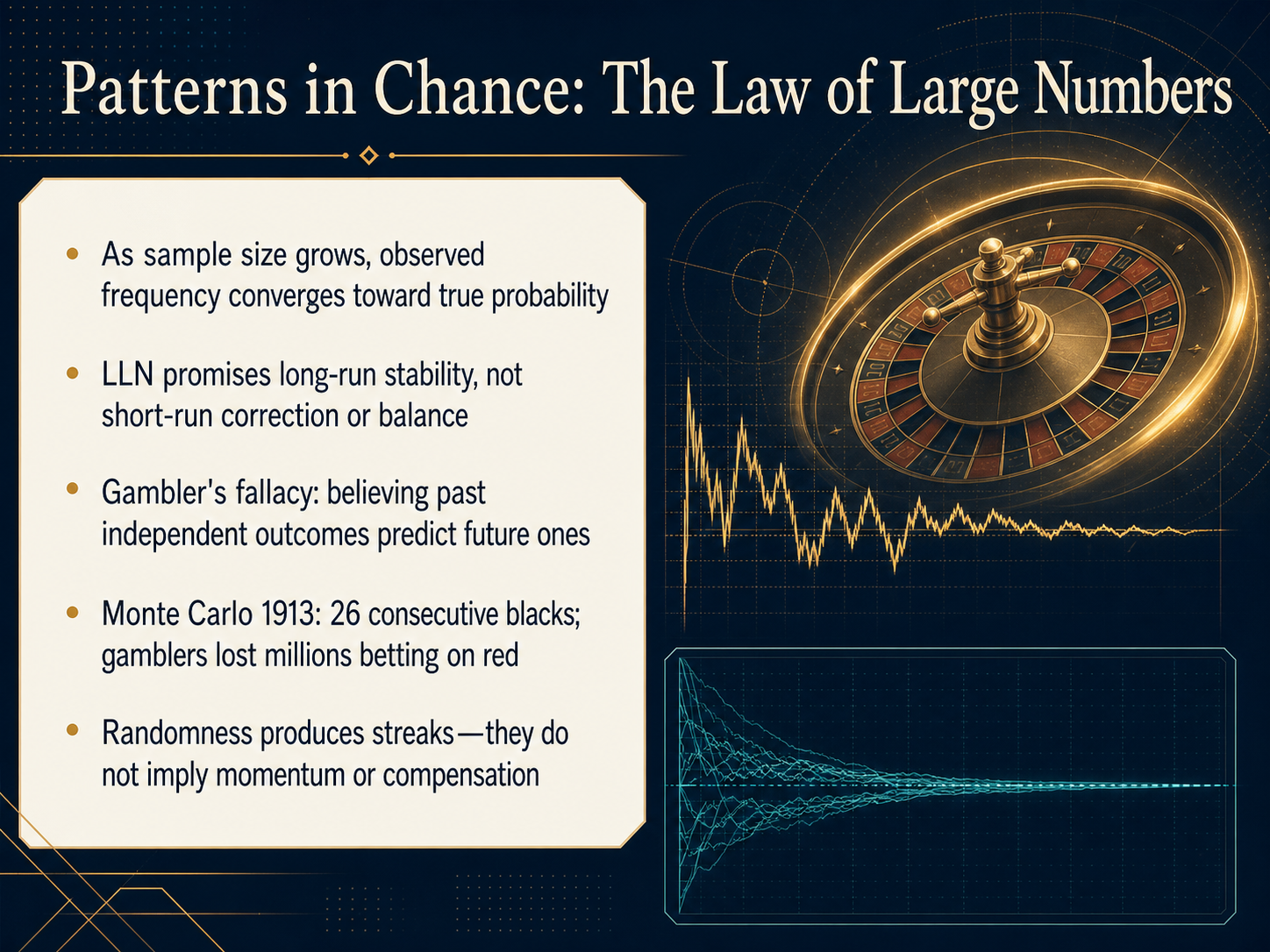
08Patterns in Chance: The Law of Large NumbersNow let's explore one of the most important patterns in chance: the Law of Large Numbers. Think of it as the mechanism that brings order to randomness over time. Imagine flipping a fair coin. After ten flips, you might see seventy percent heads. That's normal variation. But as you approach one thousand flips, the percentage of heads will be very close to fifty percent. With ten thousand flips, it'll be practically glued to the expected value. The key insight here is that the Law of Large Numbers promises long-run stability. It does not promise short-run correction. The coin has no memory, and there is no balancing force making tails 'due' after a streak of heads. This brings us to a classic trap: the gambler's fallacy. It's the mistaken belief that past independent outcomes predict future ones. A dramatic example happened at the Monte Carlo Casino in 1913, when the roulette ball landed on black 26 times in a row. Gamblers lost millions betting on red, convinced the streak had to break. In reality, randomness naturally produces streaks. They do not imply momentum, and they do not imply compensation. Up next, we'll continue this thought by discussing practical ways of avoiding the gambler's fallacy and the 'hot hand' trap.demonstrations.wolfram.com onlinemathlearning.com web-apps.thecoatlessprofessor.com+22 min
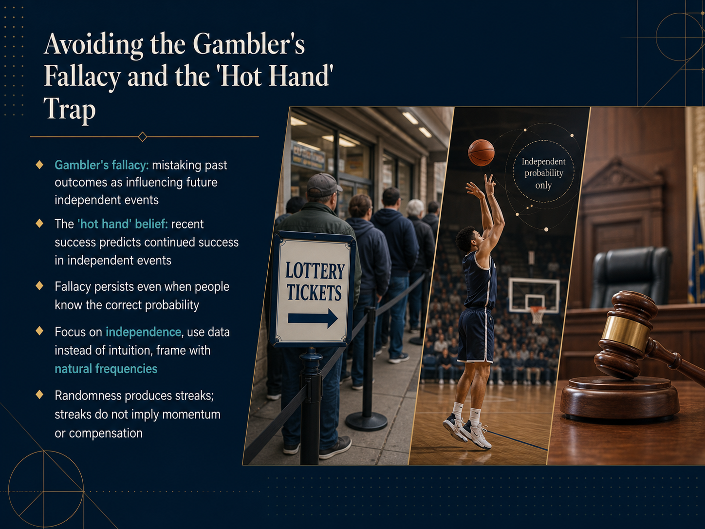
09Avoiding the Gambler's Fallacy and the 'Hot Hand' TrapLet’s move on to two common traps that can skew our judgment: the gambler’s fallacy and the hot hand belief. The gambler’s fallacy is the mistaken idea that past outcomes in independent events can somehow influence what comes next. The classic example happened at a Monte Carlo casino in 1913, when the roulette wheel landed on black 26 times in a row. Gamblers kept betting heavily on red, convinced it was ‘due.’ They lost millions. In reality, each spin is independent; the wheel has no memory. We see the same bias show up in everyday decisions—whether it’s a lottery player avoiding recent winning numbers, or a soccer goalkeeper diving the opposite way after three penalties to the same side, expecting a balance. The hot hand trap is the opposite: it’s the feeling that a streak of success means continued success, even when events are independent. Research once suggested this was an illusion in basketball, though newer studies show mixed results. But here’s the key takeaway: randomness does produce streaks. Long runs of similar outcomes are simply part of the pattern, not evidence of momentum or compensation. To avoid both fallacies, we need to focus on independence, trust data over gut feeling, and think in terms of long-run frequency rather than short sequences. Now let’s turn to a different kind of probability pitfall. 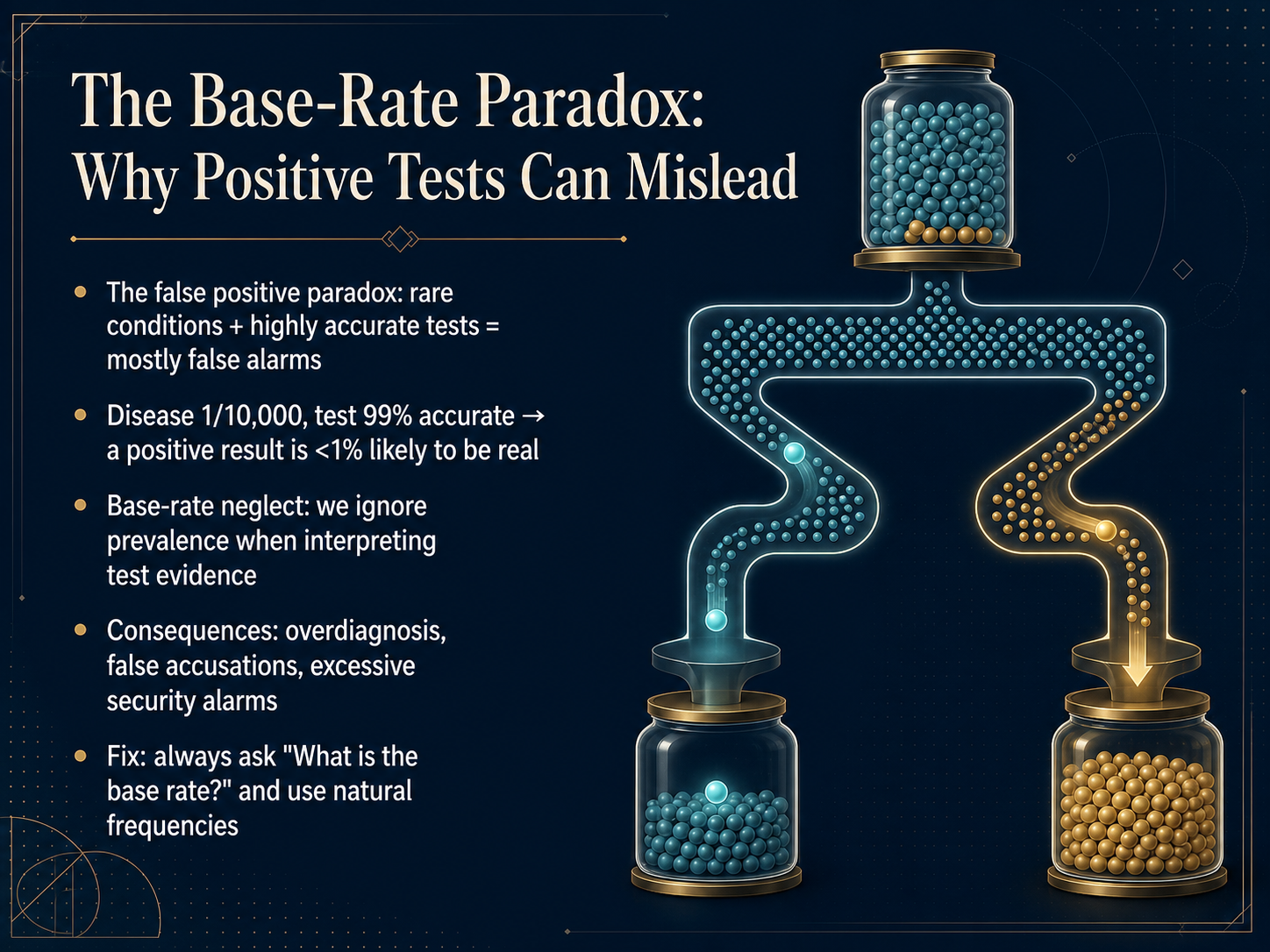Our next topic is the base-rate paradox, and why positive tests can sometimes mislead us.2 min
10The Base-Rate Paradox: Why Positive Tests Can MisleadNow let's explore a surprising paradox. Imagine a disease that affects one in ten thousand people. We have a test for it that is ninety-nine percent accurate. If you test positive, how worried should you be? Most of us feel certain we have the disease. But mathematically, a positive result means the chance you are actually sick is less than one percent. This is the false positive paradox. When a condition is extremely rare, the overwhelming majority of positive results are false alarms. The reason is base-rate neglect. Our brains fixate on the test's impressive accuracy and completely ignore how rare the condition is to begin with. Because the healthy population is so massive, even the test's tiny false-positive rate generates hundreds of false alarms that drown out the very few true cases. This isn’t just a math puzzle. It leads to overdiagnosis, unnecessary anxiety, excessive security alerts, and false accusations. The fix is to always ask a simple question. Before interpreting any result, ask yourself: What is the base rate? And frame the problem using natural frequencies. Imagine ten thousand people. Only one has the disease. The test will correctly identify that person, but it will also falsely flag about one hundred healthy people. So your positive result is just one out of a hundred and one candidates. That makes the real risk much clearer. 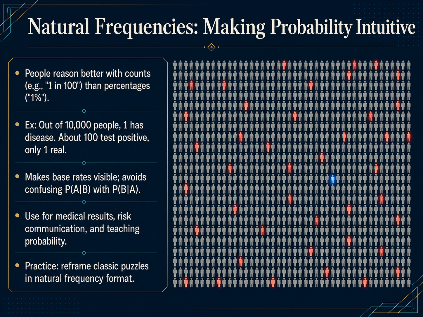Let's dive deeper into this powerful technique next, as we look at natural frequencies and how they make probability intuitive.2 min
11Natural Frequencies: Making Probability IntuitiveNow, let's make probability more intuitive. People consistently reason better with whole numbers and counts than with abstract percentages. Consider this: out of ten thousand people, only one person actually has a specific rare disease. When we test everyone, that one sick person will likely test positive. However, because the test has a small false positive rate, about one hundred healthy people will also get a positive result. So, a total of about one hundred and one people test positive, but only one of them is truly sick. This natural frequency format stops us from confusing the chance of a positive test given the disease with the chance of the disease given a positive test. It makes the base rate visible and provides a powerful tool for communicating medical results, risk, and even explaining classic probability puzzles. 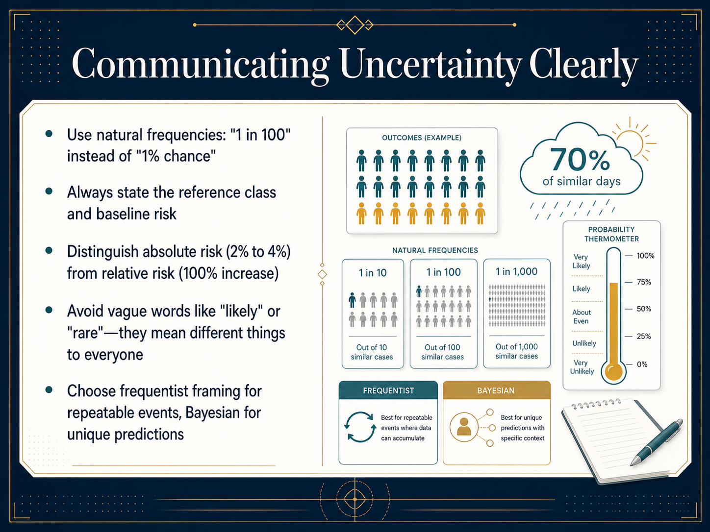Let’s now explore the next critical skill: communicating uncertainty clearly.1 min
12Communicating Uncertainty ClearlyLet's talk about how to apply our understanding of probability when it's time to communicate. The way we frame a number can dramatically change how it's understood. For example, instead of saying 'a one percent chance,' try using natural frequencies: say 'one in one hundred.' This simple shift makes the scale of the risk feel more concrete and tangible. Always remember to state the reference class. A statistic is meaningless if the audience doesn't know the baseline. Is that 'four percent' an absolute risk, or a relative increase? A jump from two percent to four percent is a modest two-percentage-point absolute increase, but it can also be framed as a 'one hundred percent' relative increase. Clearly distinguishing these prevents misinterpretation. Also, be cautious with vague words like 'likely' or 'rare.' These terms mean different things to different people, creating confusion instead of clarity. Finally, align your framing with the type of prediction. For repeatable events, like flipping a coin or running a factory machine, frequentist thinking, which relies on long-run frequency, provides clear answers. For unique predictions, like the chance of a specific project succeeding, a Bayesian approach, which updates a degree of belief with new evidence, may be a more natural fit. Choosing your words and your statistical frame intentionally helps you turn numerical uncertainty into actionable insight. Now, let's take this logic one step further by applying probability directly to everyday decisions.statsig.com thedatacopywriter.substack.com bookdown.org+22 min
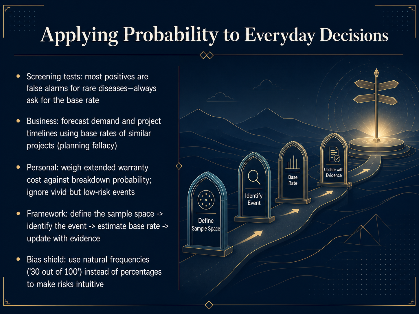
13Applying Probability to Everyday DecisionsNow let’s bring all these concepts together into a practical framework for everyday decisions. When you see a screening test result, remember the base rate. For a rare disease, most positive results are actually false alarms. Always ask what the underlying prevalence is before you worry. In business, use the same logic to forecast demand or project timelines. Look at the base rate of similar past projects to avoid the planning fallacy. For personal choices, weigh the cost of an extended warranty against the true breakdown probability, and try to ignore vivid but statistically low-risk events. Here is a simple mental checklist. First, define your sample space. Then identify the event you care about. Estimate the base rate, and only then update your estimate with new evidence. A powerful bias shield is to use natural frequencies. Think of a risk as thirty out of one hundred people, not as a percentage. This small change makes the math more intuitive and helps you avoid base rate neglect. Next, we will explore how common biases can still creep into this kind of thinking.blog.vistaslearning.com eecs70.org probability4datascience.com+22 min
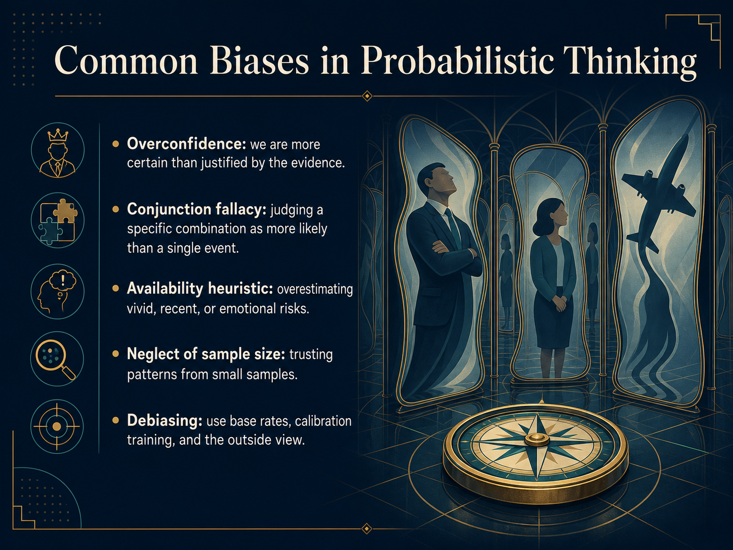
14Common Biases in Probabilistic ThinkingNow, let's turn to the common biases that can trip us up in probabilistic thinking. First, overconfidence. We are often more certain about our judgments than the evidence actually justifies. Then there is the conjunction fallacy, where we mistakenly think a specific combination is more likely than a single general event. Another trap is the availability heuristic. Vivid or emotional risks, like a recent plane crash, feel more probable, even if the base rate is extremely low. We also see neglect of sample size. People often trust a clear pattern from just a handful of examples, ignoring the fact that small samples are highly variable. To debias our thinking, start by always asking for the base rate. Use calibration training to align your confidence with your actual accuracy. And adopt the outside view by grounding your estimate in what happened with similar situations, not just the specifics of the current case. Understanding these biases gives you a practical toolkit for making more realistic probability judgments in your daily work.stat.berkeley.edu link.springer.com stats.stackexchange.com+22 min
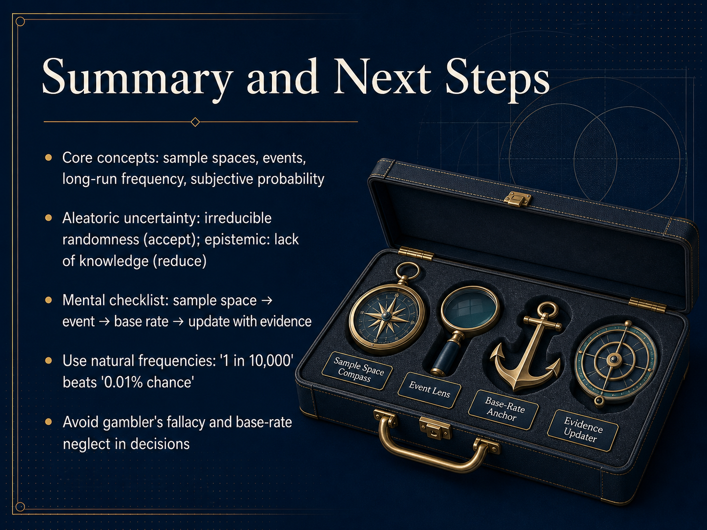
15Summary and Next StepsLet's quickly recap the toolkit we've built for thinking about chance. We start by mapping the sample space, which is the set of all possible outcomes, and then defining our event of interest. The probability of that event is its long-run frequency over many, many repetitions. Remember that not all uncertainty is the same. Aleatoric uncertainty is the irreducible randomness, like a fair coin flip, and we learn to accept it. Epistemic uncertainty, on the other hand, comes from a lack of knowledge, like an estimate we can improve with more research, so we work to reduce it. To avoid mistakes, use a mental checklist: define the sample space, then the event, then lock in the base rate before you update that number with new evidence. Communicate these numbers as natural frequencies. Saying 'one in ten thousand' is much clearer and prevents the base-rate neglect that often misleads people. Finally, watch out for the gambler's fallacy. A roulette wheel has no memory, and a streak does not make a different outcome 'due'. You now have a robust framework for navigating uncertainty with clarity and confidence. Thank you for joining me, and I look forward to seeing you apply these concepts in your own decision-making.stat.berkeley.edu link.springer.com stats.stackexchange.com+22 min

Sources consulted

Web sources consulted while building this course.