Understanding Variance in Statistics

What you’ll learn

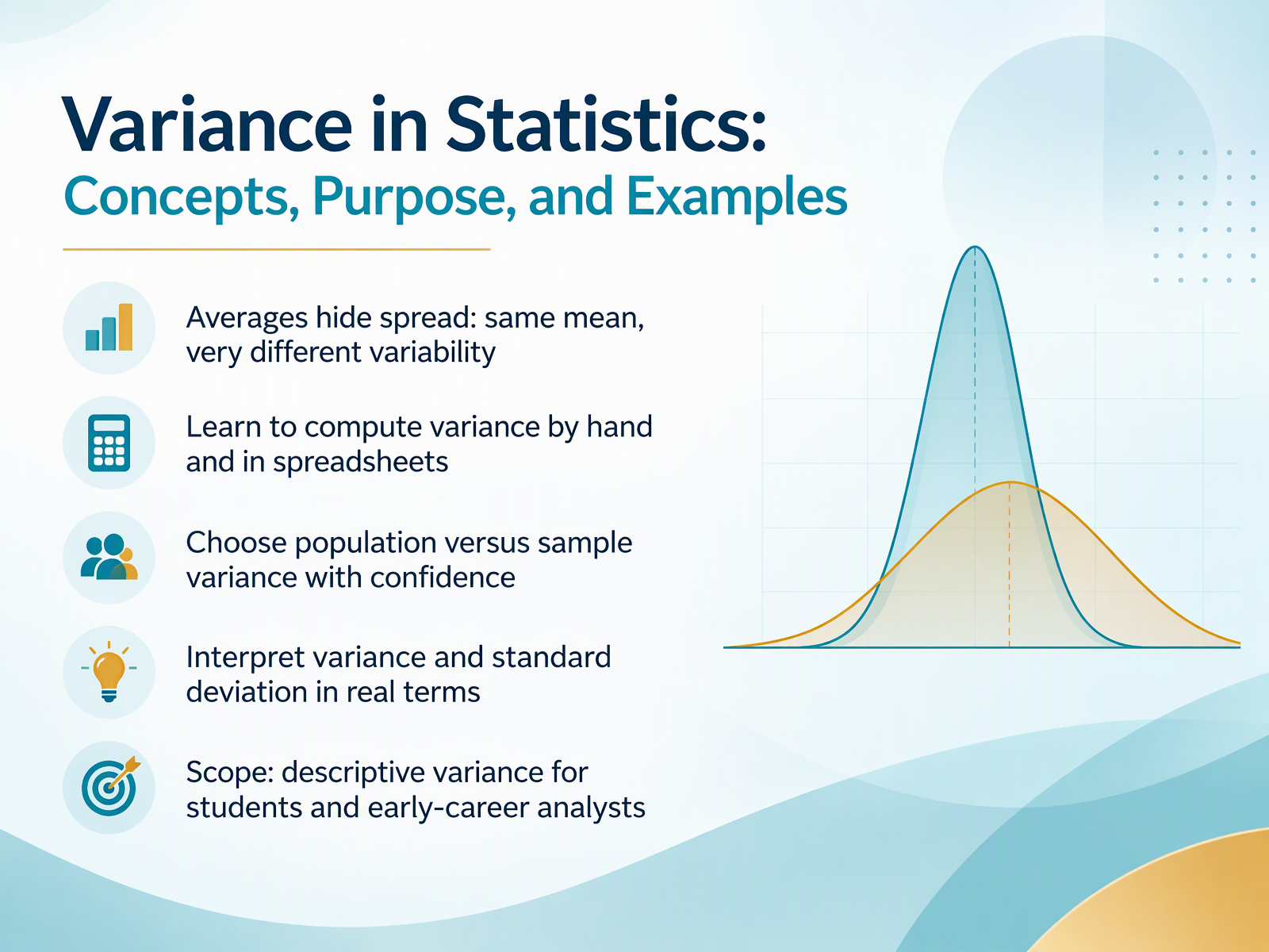
1. 01Variance in Statistics: Concepts, Purpose, and ExamplesWelcome. I'm glad you're here. Today we're going to build a clear, practical understanding of variance in statistics. You already know how to work with averages, and that's a great foundation. Our goal is to help you see what an average can hide, and to give you a reliable way to measure spread. By the end of this course, you'll be able to compute variance by hand and in a spreadsheet, choose between population and sample variance with confidence, and interpret variance and standard deviation in real terms. We'll keep the scope focused on descriptive variance for students and early-career analysts. Here's a quick preview of the central idea. Two groups can share the same mean yet have very different variability. Averages hide spread, and variance makes that spread visible. So let's begin by asking why averages alone are not enough.2 min
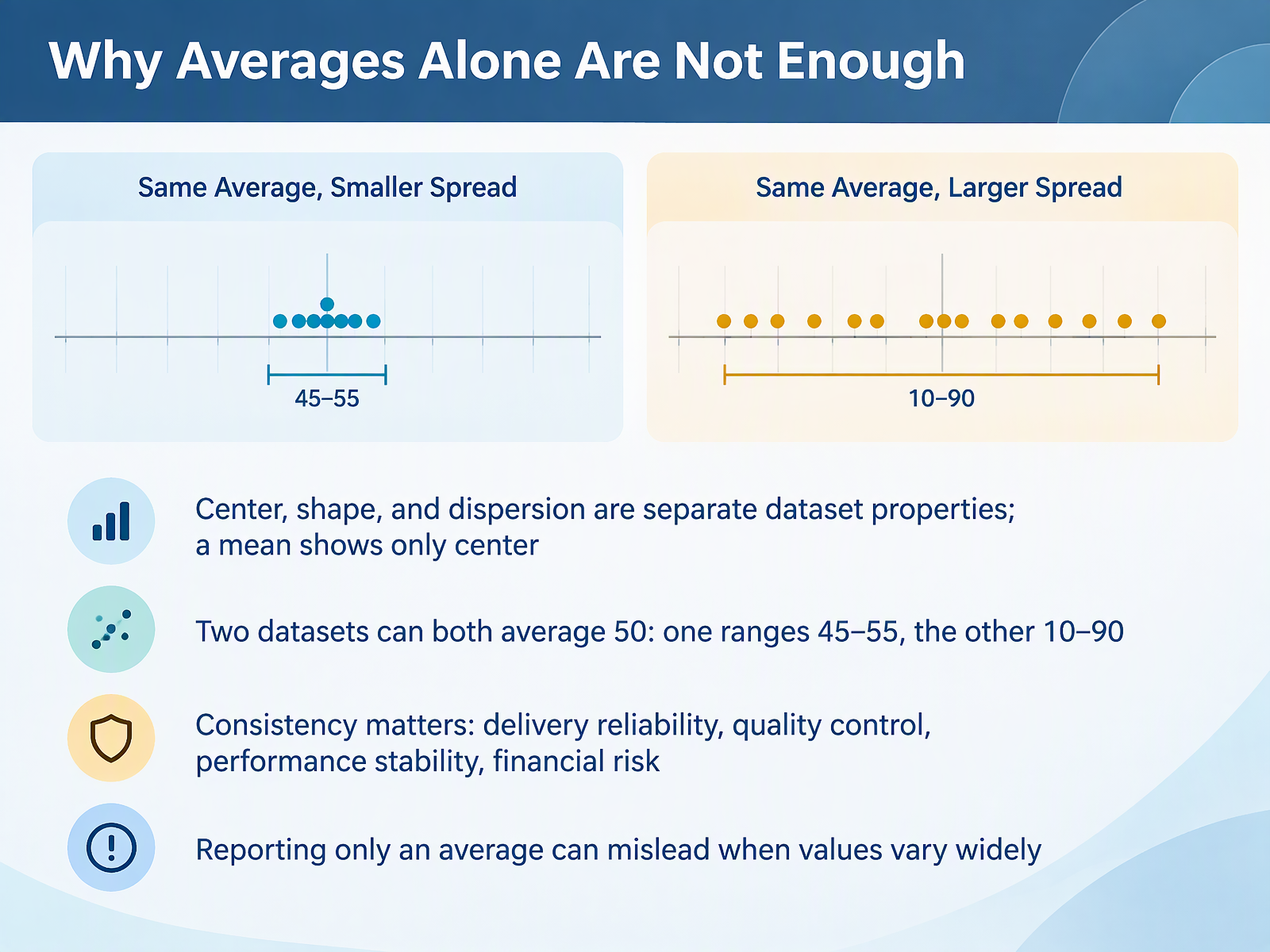
2. 02Why Averages Alone Are Not EnoughLet's take the next step. Why don't averages alone tell the full story? Here's the key idea. Center, shape, and dispersion are three separate properties of a dataset. A mean describes only the center. It tells you nothing about how spread out the values are. Consider two datasets. Both average fifty. In the first, values range from forty five to fifty five. In the second, values range from ten to ninety. Same mean, very different stories. Notice that consistency matters in real work. Think about delivery reliability, quality control, performance stability, and financial risk. In each case, an average hides the variation that actually drives decisions. Here's why that matters. Reporting only an average can mislead when values vary widely. So as you work through variability, keep asking what the spread adds to the picture. Next, we'll look at deviations from the mean.1 min
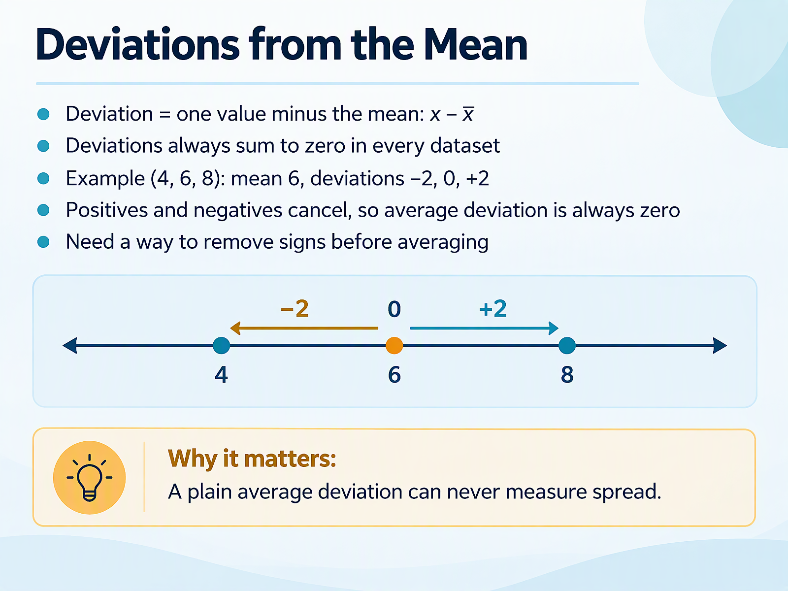
3. 03Deviations from the MeanNow that you're comfortable thinking in terms of averages, let's look at what happens when individual values move away from the mean. We call this a deviation. It's simple: take one value and subtract the mean, so the deviation equals x minus x bar. For our example with the values four, six, and eight, the mean is six. So the deviations are negative two, zero, and plus two. Notice the pattern: the negative and positive values cancel each other out, which means deviations always sum to zero in every dataset. That makes sense, but here's why it matters. If you average those deviations, you always get zero, so a plain average deviation can never measure spread. It tells you nothing about how far the values really are from the mean. So we need a way to remove those signs before averaging. In the next slide, we'll look at squaring deviations and the sum of squares.1 min
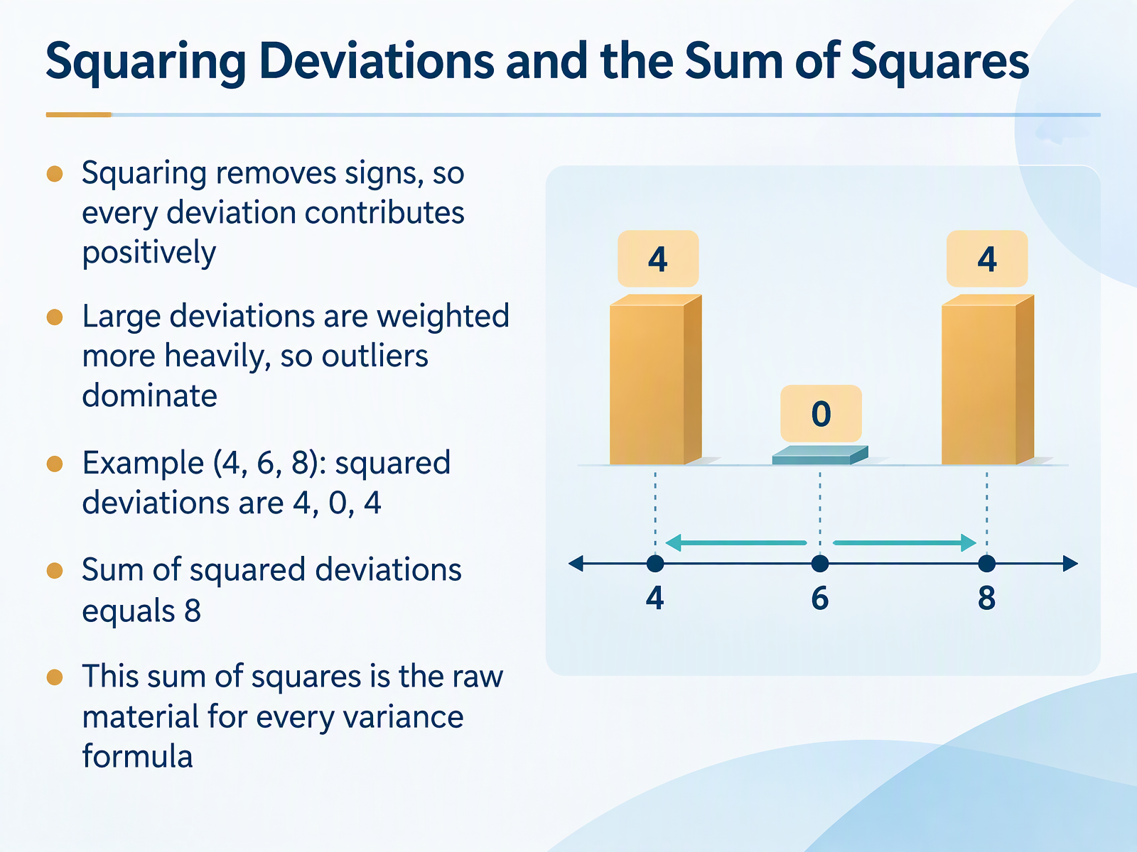
4. 04Squaring Deviations and the Sum of SquaresNow that you have deviations, the next step is to square them. Squaring does two things for you. First, it removes the signs, so every deviation contributes positively to the total. Second, it weights larger deviations more heavily. A deviation of four becomes sixteen, while a deviation of two becomes just four. Notice that outliers can dominate this measure. Here's why that matters when you interpret results. Let's apply this to the numbers four, six, and eight. The mean is six. The deviations are negative two, zero, and positive two. Squared, they become four, zero, and four. Add those up and the sum of squared deviations equals eight. This sum of squares is the raw material for every variance formula you will use. In the next slide, we turn it into the variance formula for populations versus samples.1 min
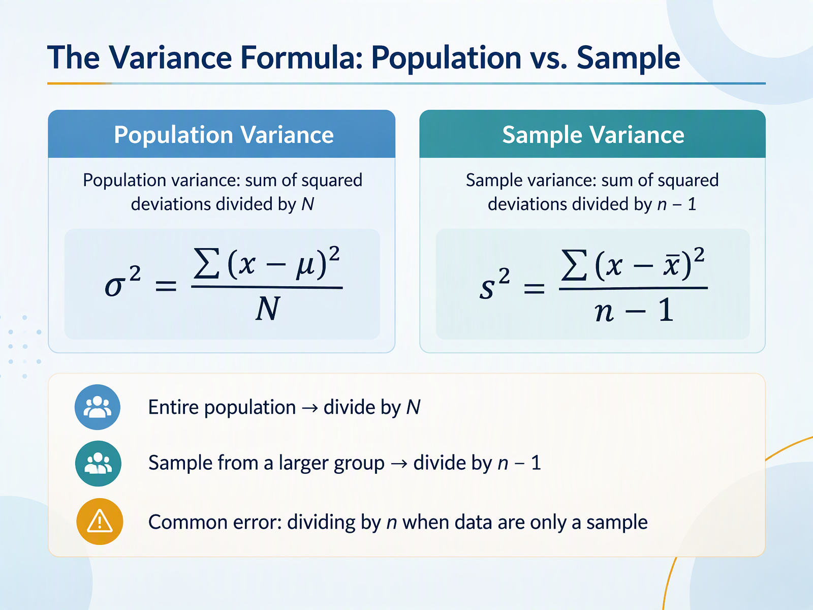
5. 05The Variance Formula: Population vs. SampleNext, let's put the variance idea into its two formulas. For a population, you take the sum of the squared deviations and divide by capital N, the total number of values in that population. When you only have a sample from a larger group, you divide by n minus one instead of n. Here's why that matters. The sample mean is drawn from the same data, so it tends to sit closer to the center, and dividing by n minus one corrects that tendency and gives a more honest estimate of the population variance. A common error is dividing by n when your data are only a sample. Notice the question to ask yourself: do I have the entire population, or just a sample? That answer decides which denominator you use. Up next, we explain why we divide by n minus one.1 min
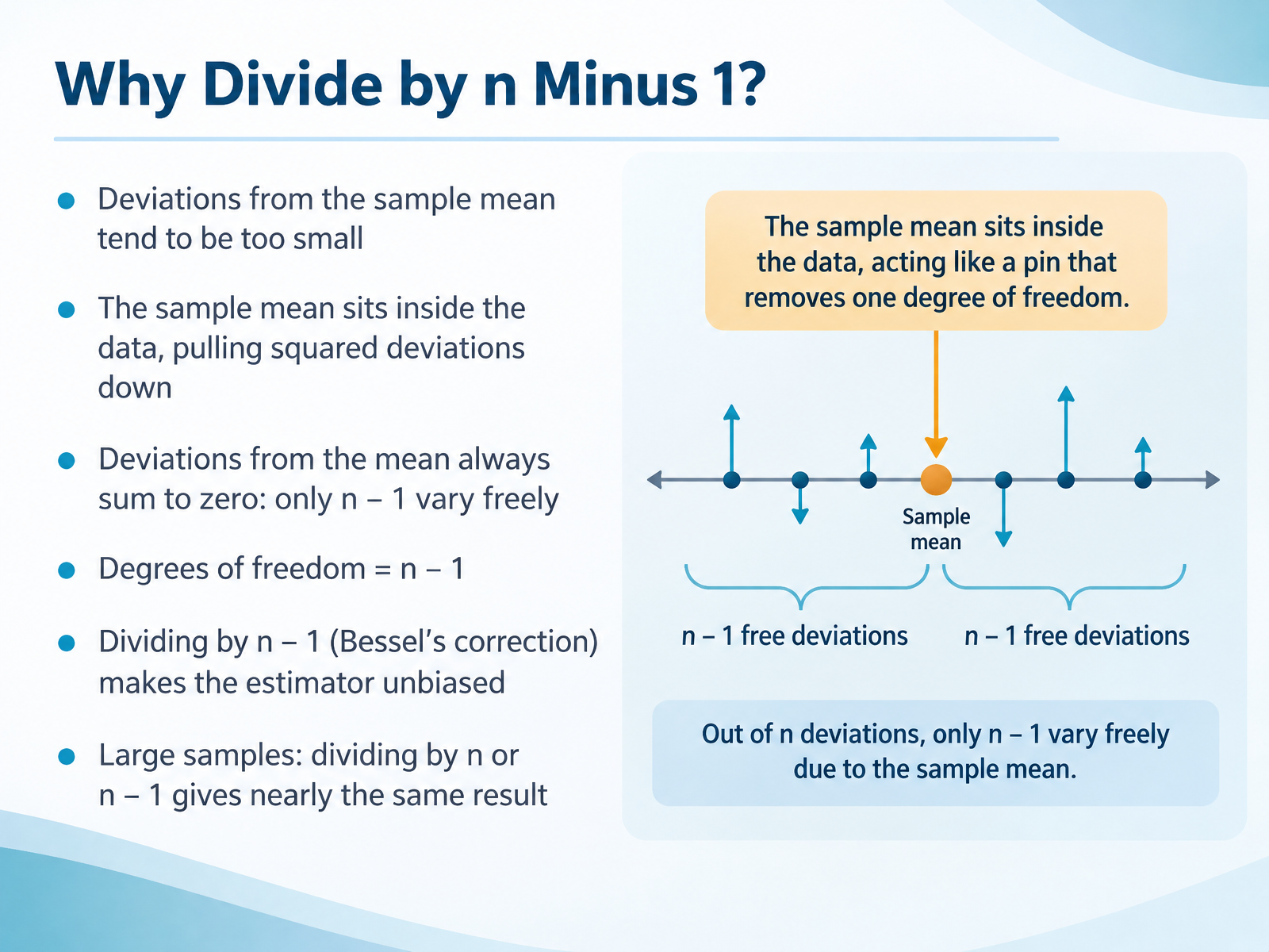
6. 06Why Divide by n Minus 1?Now let's answer a question you've likely wondered about. When we calculate sample variance, why do we divide by n minus 1 instead of just n? Here's the intuition. Deviations from the sample mean tend to be too small, because the sample mean sits inside your data and pulls those squared deviations down. In fact, deviations from the mean always sum to zero. So once you know n minus 1 of them, the last one is fixed. Only n minus 1 values vary freely. That number is called degrees of freedom. Dividing by n minus 1, known as Bessel's correction, makes the estimator unbiased. And notice this. With large samples, dividing by n or by n minus 1 gives nearly the same result. Next, let's put this into practice with a worked example, variance step by step.1 min
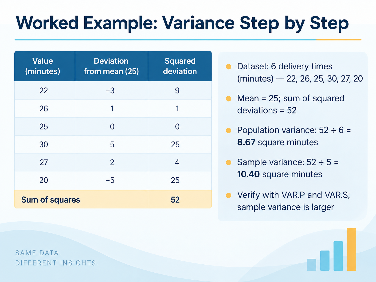
7. 07Worked Example: Variance Step by StepNow let's work through variance step by step with a real dataset. You have six delivery times in minutes: twenty-two, twenty-six, twenty-five, thirty, twenty-seven, and twenty. First, find the mean. The sum is one hundred fifty, and one hundred fifty divided by six equals twenty-five. Next, subtract the mean from each value. You get negative three, one, zero, five, two, and negative five. Notice the positives and negatives cancel out, so we square each deviation: nine, one, zero, twenty-five, four, and twenty-five. The sum of squared deviations is fifty-two. Here's why that matters. For population variance, divide by six: fifty-two divided by six equals eight point six seven square minutes. For sample variance, divide by five, because you subtracted one degree of freedom for the mean: fifty-two divided by five equals ten point four zero square minutes. To verify, use V A R dot P for population and V A R dot S for sample. And notice the sample variance is larger, which is expected. Next, we'll see how to verify these results in a spreadsheet.2 min
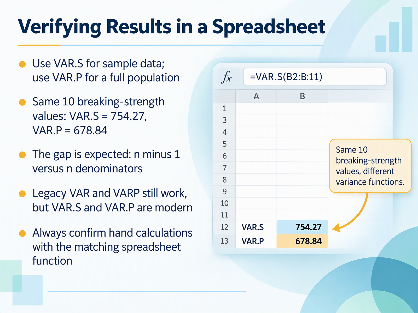
8. 08Verifying Results in a SpreadsheetNext, let's verify your results using a spreadsheet. When your data is a sample, use the function VAR.S. When you have the entire population, use VAR.P. We'll use the same ten breaking-strength values. In the spreadsheet, VAR.S gives 754.27, and VAR.P gives 678.84. Notice the gap between them. That's expected, because the sample version divides by n minus one, while the population version divides by n. The smaller denominator makes the sample variance a bit larger. You may also see the older functions VAR and VARP. They still work, but VAR.S and VAR.P are the modern choices. So here's a practical habit: after you calculate variance by hand, confirm it with the matching spreadsheet function. That catches arithmetic slips and denominator mistakes. Coming up, we'll look at interpreting variance and standard deviation.1 min
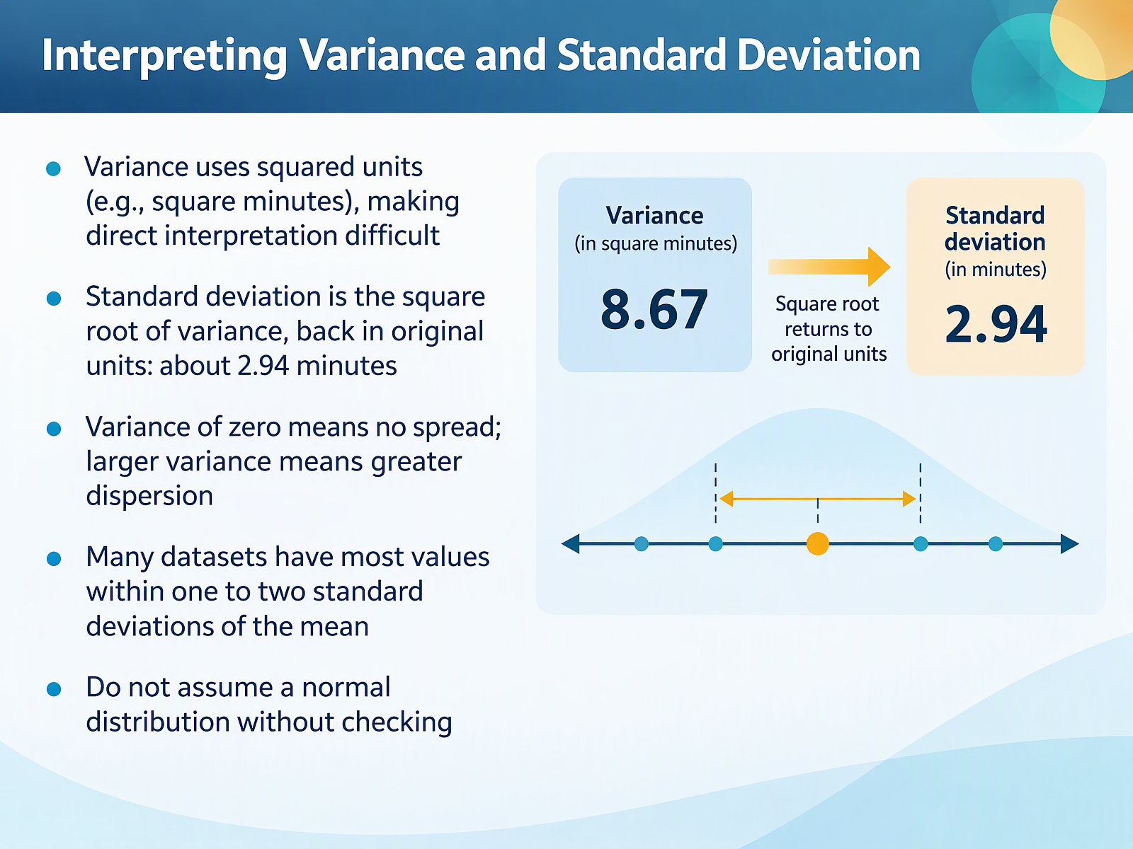
9. 09Interpreting Variance and Standard DeviationNow let's talk about interpreting variance and standard deviation. Remember that variance uses squared units, such as square minutes. Notice that this makes direct interpretation difficult, because square minutes don't describe the spread in a way most people can picture. That's exactly why standard deviation matters. It's the square root of the variance, so take the square root of ten point eight, and you get about two point nine four minutes. The result is back in the original units. Here's why that matters: two point nine four minutes is easy to compare with the mean, and easy to explain to someone else. Keep two quick rules in mind. A variance of zero means no spread at all, while a larger variance means greater dispersion. In many datasets, most values fall within one to two standard deviations of the mean, but do not assume a normal distribution without checking. Real data can be skewed or have outliers, so always visualize before relying on that pattern. Next, we look at comparing variability across groups.2 min
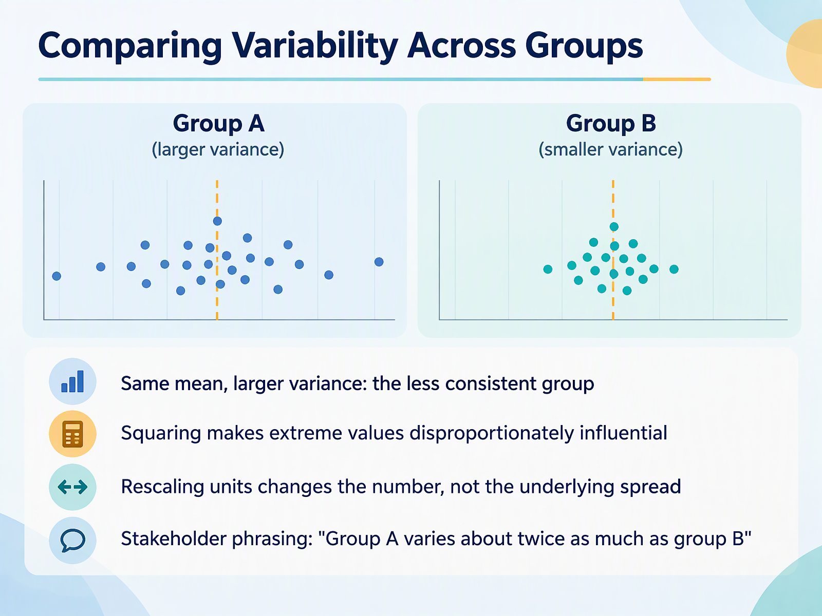
10. 10Comparing Variability Across GroupsNow let's compare variability across groups. Imagine two groups with exactly the same mean. If one group has a larger variance, that group is the less consistent one. Its values scatter further from the average. Notice that the mean alone would not reveal this. Squaring the deviations is also why extreme values matter so much here. A value twice as far from the mean contributes four times as much to the variance, so one outlier can inflate the number quickly. Also, if you rescale the units, say from dollars to thousands of dollars, the variance number changes, but the underlying spread does not. Here is why that matters for stakeholders. A clear phrasing is, Group A varies about twice as much as group B. That sentence compares spread directly, without leading with technical terms. Next, we look at the limits of variance and complementary measures.1 min
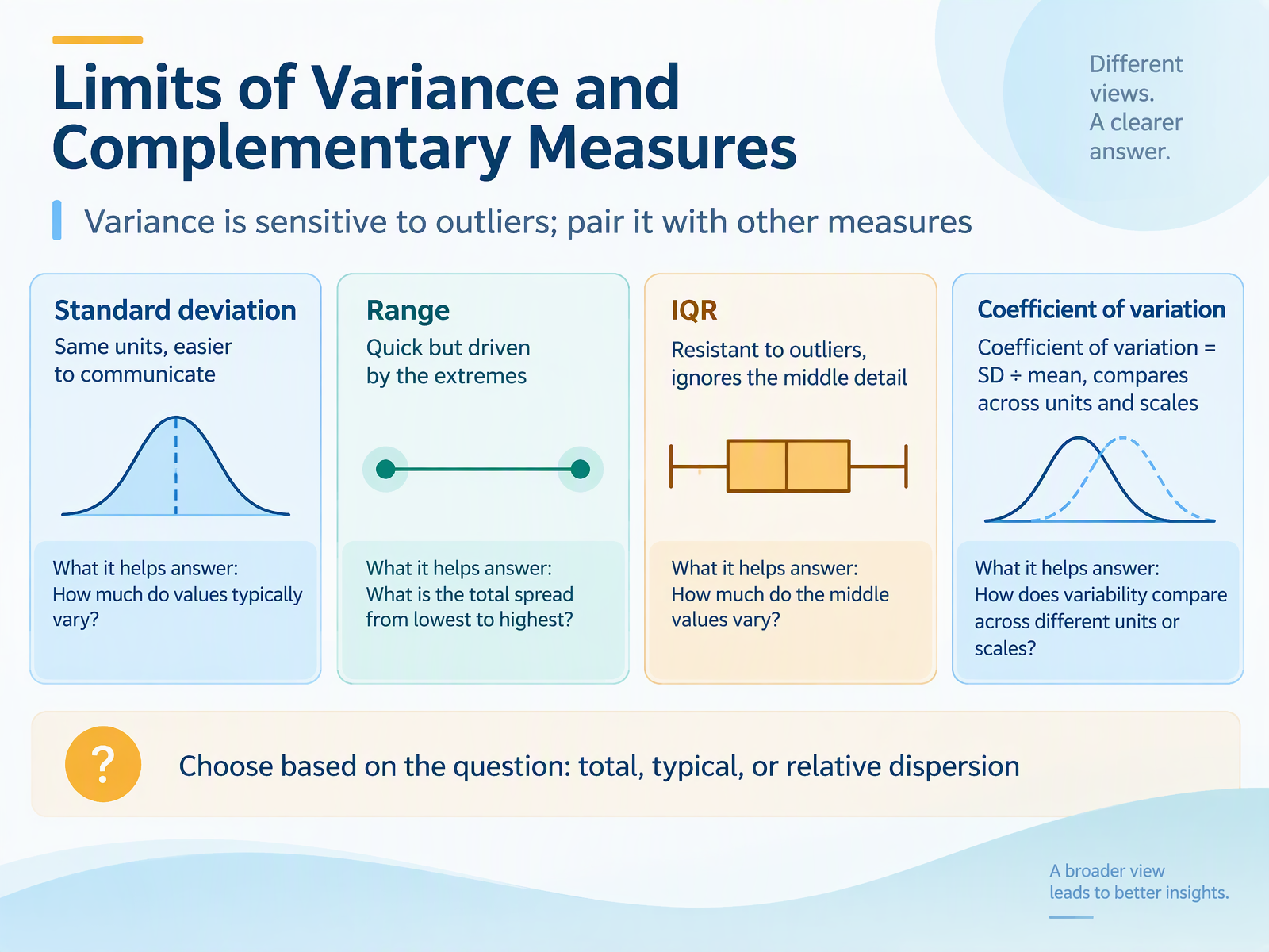
11. 11Limits of Variance and Complementary MeasuresNow that you can compute variance, let's talk about where it has limits, and which measures can fill the gaps. Variance is sensitive to outliers. Notice that one extreme value can pull the mean, and therefore the variance, far away from the rest of the data. So pair it with other measures. Standard deviation is in the same units as your data, which makes it easier to communicate. Range is quick to calculate, but it is driven entirely by the extremes. The interquartile range, or I Q R, is resistant to outliers because it focuses on the middle half of the data, though it ignores detail within that middle. The coefficient of variation equals the standard deviation divided by the mean. Here's why that matters: it lets you compare variability across different units and scales. For example, a standard deviation of ten may be large for one data set and small for another. The coefficient of variation puts that in relative terms. So choose based on the question. Do you need total dispersion, typical spread, or relative spread? That choice tells you which measure to report. Next, let's look at common mistakes to avoid.1 min
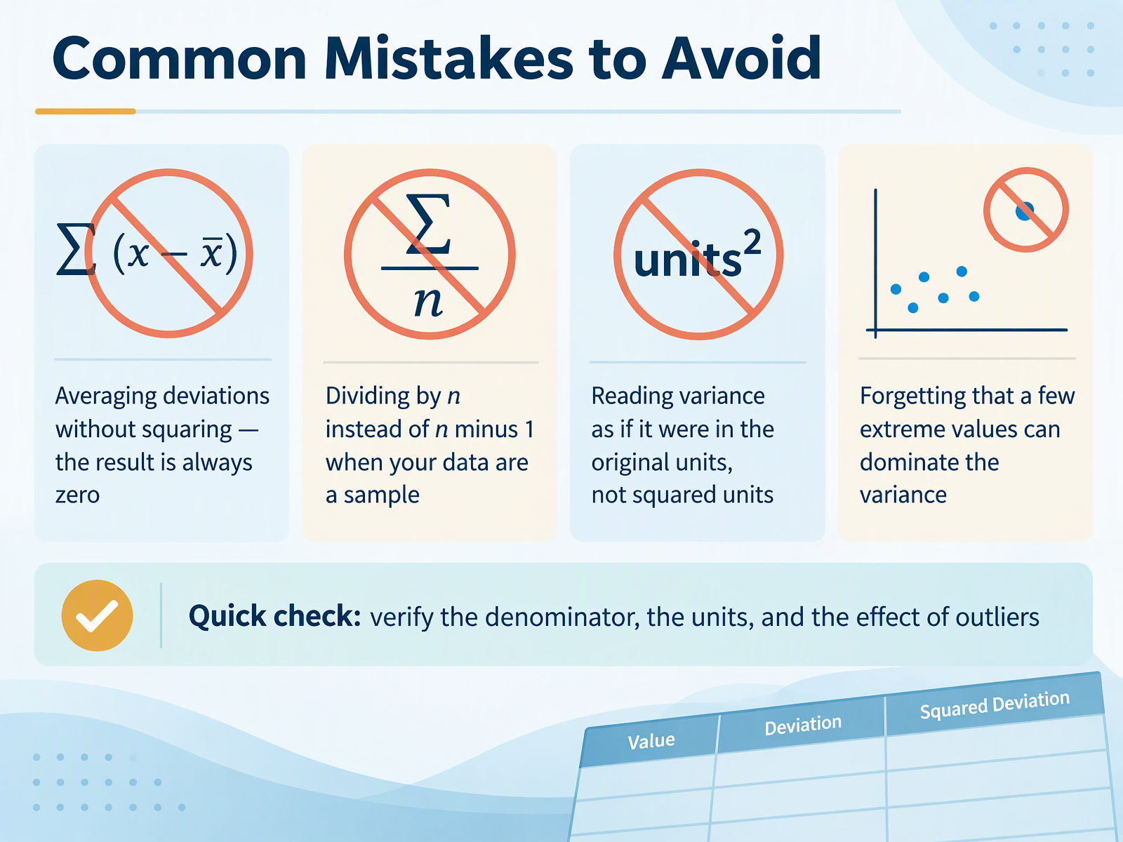
12. 12Common Mistakes to AvoidLet's turn to common mistakes to avoid. These are the places where careful analysts still slip, so check your own work against each one. First, averaging deviations without squaring. If you add up each value minus the mean and divide, the result is always zero. The positives and negatives cancel. That is exactly why we square deviations first. Second, dividing by n instead of n minus 1 when your data are a sample. Using n underestimates the variability in the population. For a sample, use n minus 1. Third, reading variance as if it were in the original units. If your data are in dollars, variance is in dollars squared. That is why we often take the square root to get standard deviation. Fourth, forgetting that a few extreme values can dominate the variance. Notice that squaring gives outliers extra weight. One very large value can inflate the result dramatically. Here is a quick check before you finish. Verify the denominator, check the units, and think about the effect of outliers. Now let's put this into practice with Quick Practice and Self-Check.2 min
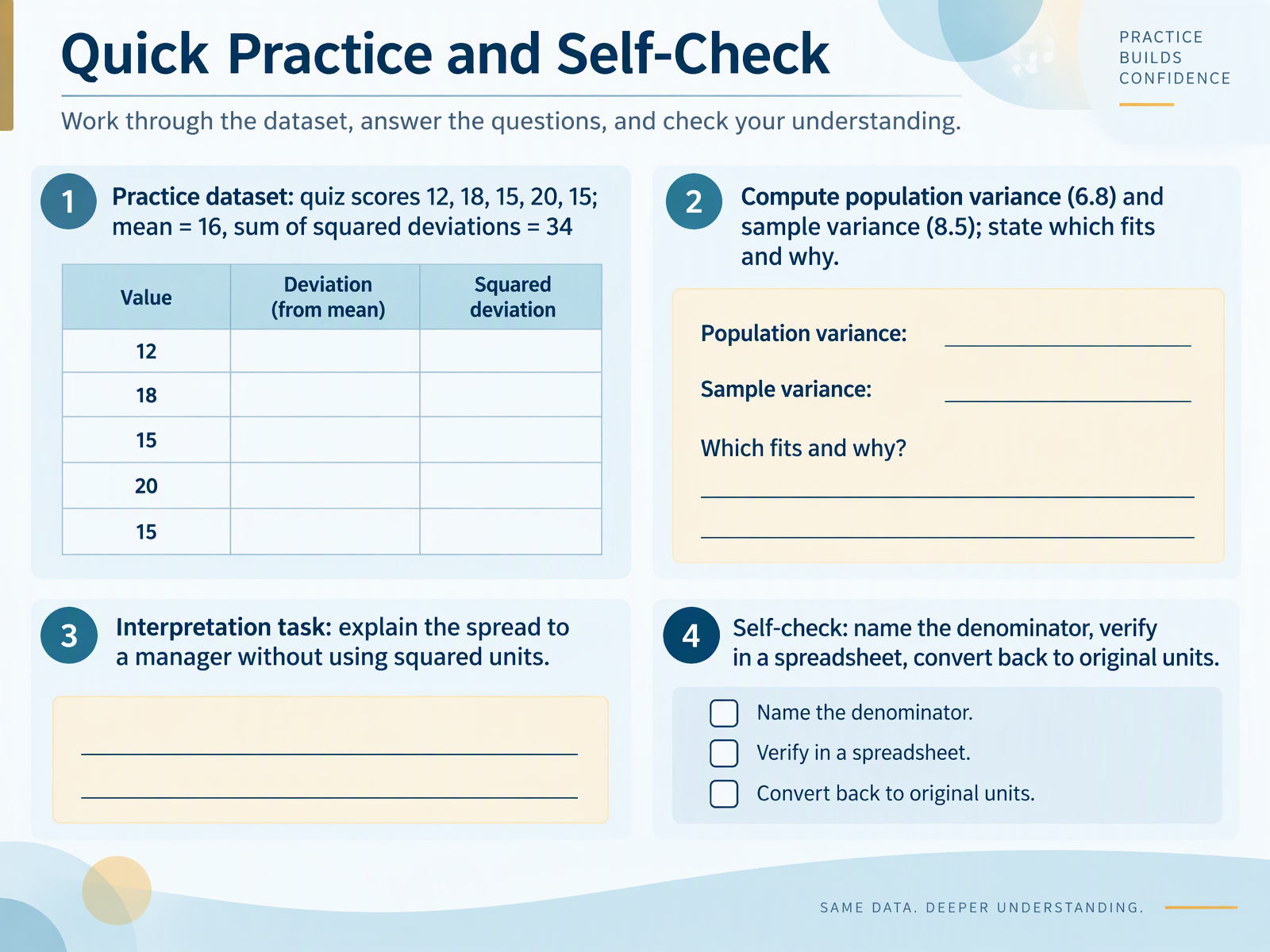
13. 13Quick Practice and Self-CheckLet's put this into practice with a quick self-check. Here is a small quiz dataset: twelve, eighteen, fifteen, twenty, and fifteen. The mean is sixteen, and the sum of squared deviations is thirty-four. First, compute the population variance by dividing thirty-four by five. That gives six point eight. Now compute the sample variance by dividing thirty-four by four. That gives eight point five. Which one fits? If these scores are your entire group, use the population variance. If they are a sample used to estimate a wider group, use the sample variance. Here's why that matters: the sample formula divides by one fewer value, so it is slightly larger, which helps correct for estimating from limited data. For interpretation, avoid squared units. Tell your manager the scores typically sit about two point six points from the mean, since the square root of six point eight is roughly two point six. That is a standard deviation, back in the original quiz-score units. Now a quick self-check: can you name the denominator for each variance? Five for population, four for sample. Then verify the numbers in a spreadsheet, and convert the result back to original units. In the next slide, we'll bring it all together with key takeaways and next steps.2 min
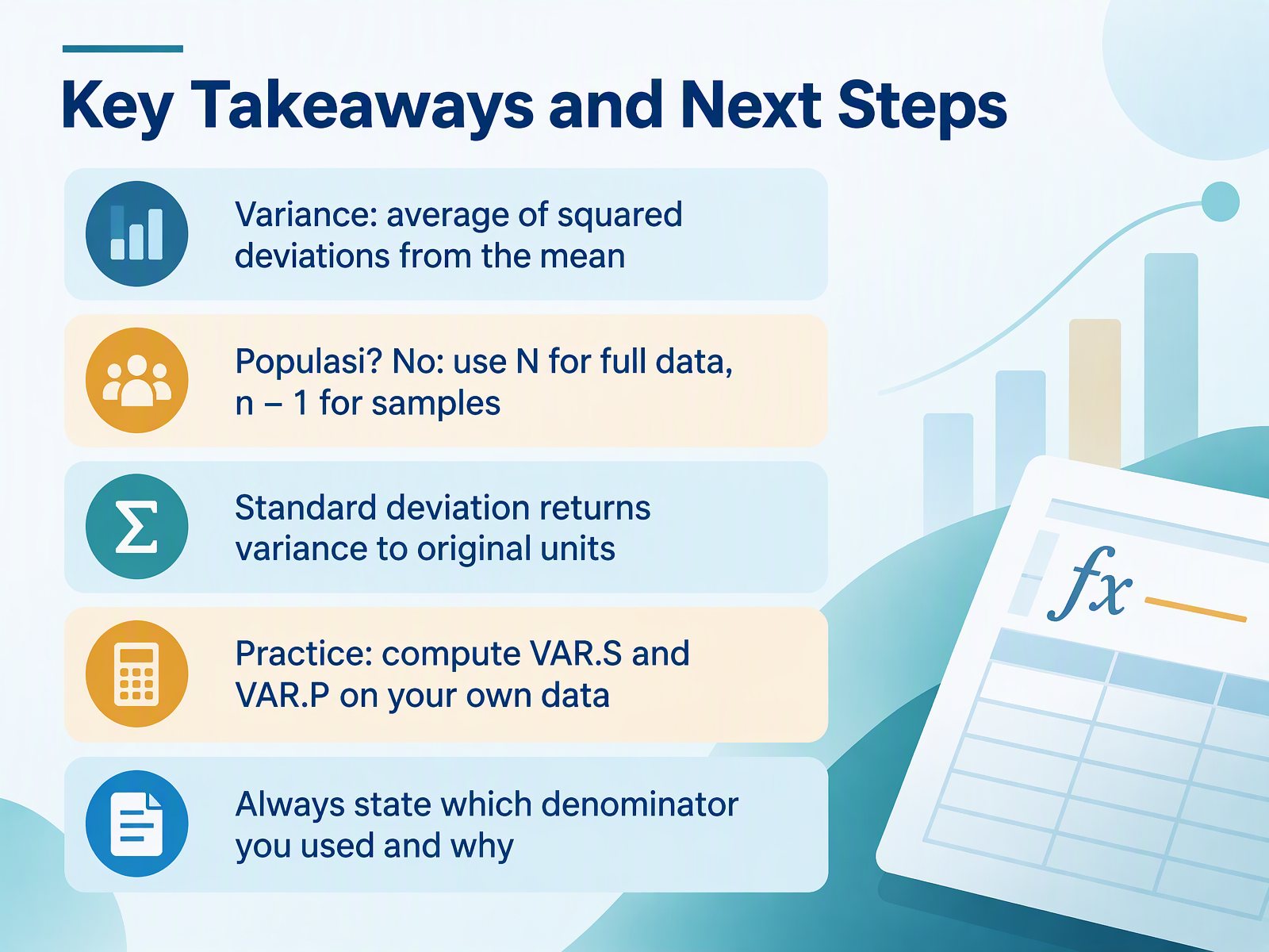
14. 14Key Takeaways and Next StepsLet's pull together what you've learned. Variance is the average of the squared deviations from the mean. It tells you how spread out your data is, in squared units. Now, which denominator do you use? If you have the full population, divide by capital N. If you have a sample and want to estimate the population variance, divide by n minus one. That adjustment corrects for the fact that a sample tends to underestimate spread. Standard deviation simply takes the square root of variance, returning you to the original units, which makes it easier to interpret. Here's your next step: practice computing variance on your own data using the sample and population functions in your spreadsheet, and compare the results. Notice how the sample variance is slightly larger. Always state which denominator you used and why, because that choice matters for interpretation. You've built a solid foundation. Thank you for your attention, and keep exploring your data with confidence.1 min

Take the deck with you

Download this course as a file — free, no sign-up needed.

• PDF handoutEvery slide page, ready to print or share.15 pages · 2.9 MBDownload
• Narrated PowerPointThe deck that presents itself — every slide carries the digital human's narration video.15 pages · 12.1 MBDownload
• PowerPoint slidesThe full deck as a .pptx — open it in PowerPoint, Keynote, or Google Slides.15 pages · 2.8 MBDownload

Free to use in your own training — please keep the PersonWise credit page at the end.

Have your own deck? Turn it into a course