The instructor is ready

Algorithms Fundamentals

Interactive digital-human course

Algorithms Fundamentals

Name: Algorithms Fundamentals
Availability: InStock

This training introduces the fundamental concepts of algorithms, aimed at beginners seeking to understand how algorithms work and their role in problem-solving.

My workspace32 minFree to watch

What you’ll learn

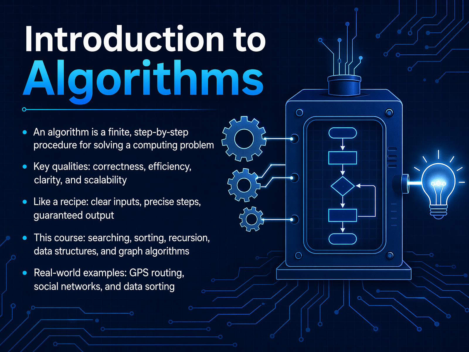
01Introduction to AlgorithmsWelcome to Introduction to Algorithms. If you already write a bit of code, you know how to make a computer do things. But an algorithm is more than just code. It is a finite, step-by-step procedure for solving a computing problem. Think of it like a recipe. A recipe takes clear inputs, follows precise steps, and gives you a guaranteed output. A good algorithm does the same, but it also needs to be correct, efficient, clear, and able to scale up when the problem gets bigger. In this course, we will walk through searching, sorting, recursion, data structures, and graph algorithms. These are the building blocks behind tools you use every day, like GPS routing, social networks, and data sorting. By the end, you will see algorithms not as abstract theory, but as practical, logical tools you can control. Let's get started by defining exactly what an algorithm really is.britannica.com simple.wikipedia.org mathwords.com+21 min
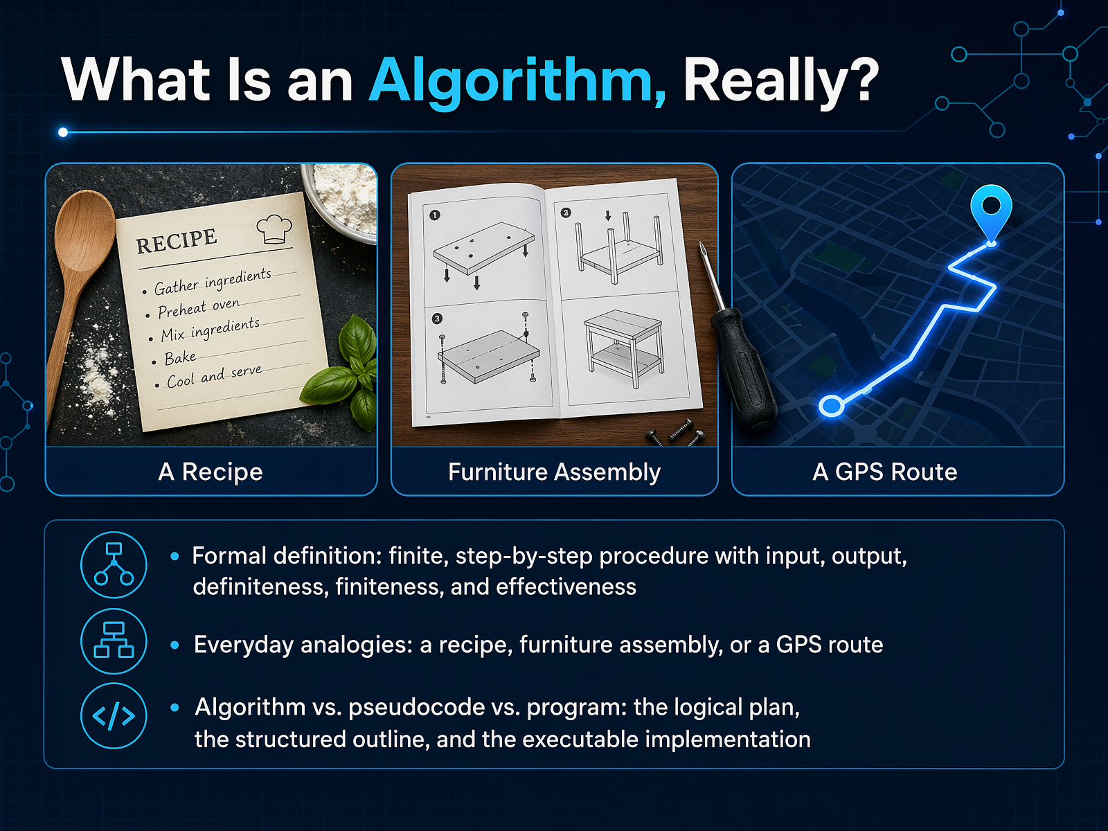
02What Is an Algorithm, Really?Now let’s get precise: what is an algorithm, really? Formally, it’s a finite, step‑by‑step procedure that has clear inputs, produces a clear output, and follows five key properties. Each step must be definite—no ambiguity. The process must be finite, meaning it eventually stops. And it must be effective, so each step is actually doable. You already know this pattern from everyday life. A recipe is an algorithm: you start with ingredients, follow ordered steps, and end with a dish. Furniture assembly instructions guide you from a box of parts to a finished product. A GPS route takes your start and destination, then computes turn‑by‑turn directions. The same logic applies in computing. Notice the difference between an algorithm, pseudocode, and a program. An algorithm is the logical plan—the what and why. Pseudocode is a structured, language‑neutral outline of that plan. A program is the executable implementation written in a specific language like Python or Java. Keep this separation in mind, because it helps you design before you code. Next, we’ll explore why algorithms are the core of computing.britannica.com simple.wikipedia.org mathwords.com+22 min
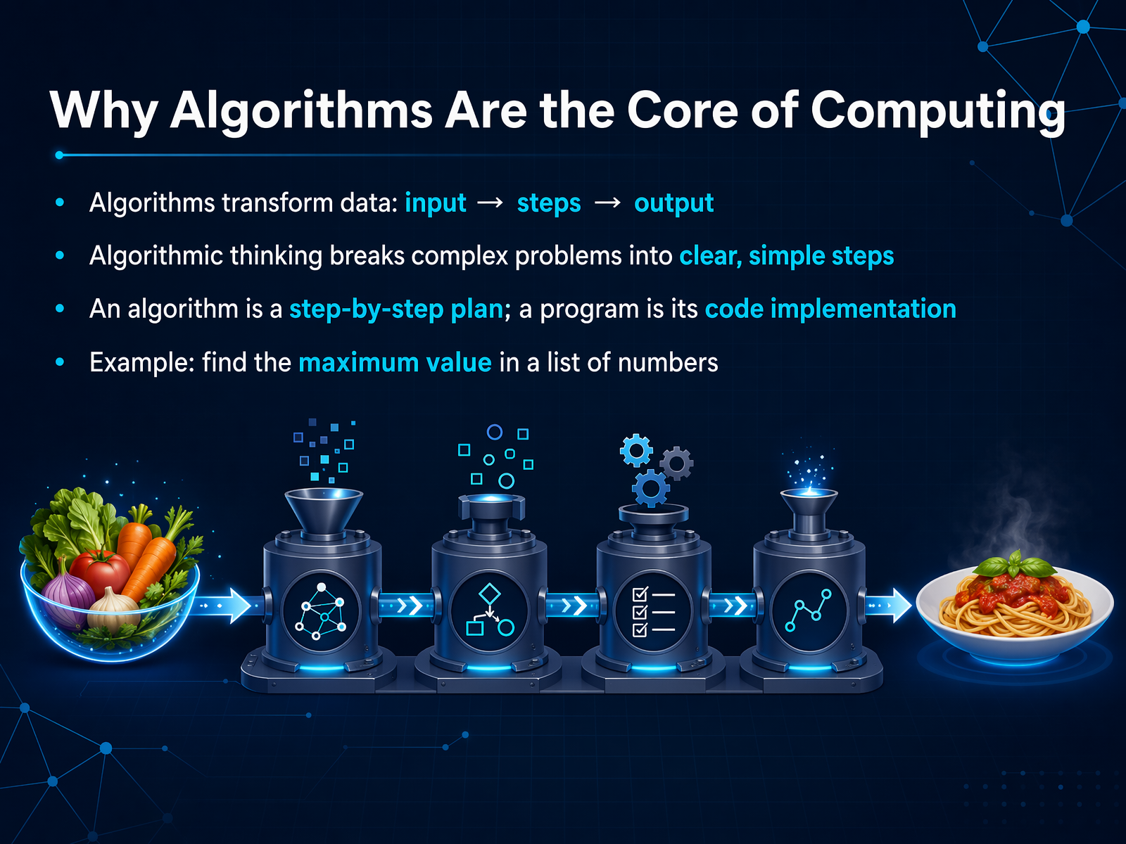
03Why Algorithms Are the Core of ComputingNow that we understand the basic idea, let's look at why algorithms are the core of computing. Think of an algorithm as a precise plan, and a program as the finished house built from that blueprint. An algorithm transforms data through a clear pattern: you have an input, a series of defined steps, and an output. It's a high-level, logical description that breaks complex problems into simple, manageable actions. Algorithmic thinking is exactly that—taking a big challenge and dividing it into a sequence of small, unambiguous instructions. The algorithm itself is language-agnostic; it's the step-by-step plan. A program is the concrete implementation of that plan, written in a specific language like Python so a machine can actually execute it. For example, let's take the problem of finding the maximum value in a list of numbers. The algorithm would be: start by assuming the first number is the largest, then look at each remaining number one by one, and if you find a bigger one, update your assumption. That's the logic. The program is the actual code that loops through the list and performs those comparisons. Up next, we'll explore how to measure the efficiency of these plans in our section on Measuring Efficiency: Time and Space Complexity.scribbr.com en.wikibooks.org geeksforgeeks.org+22 min
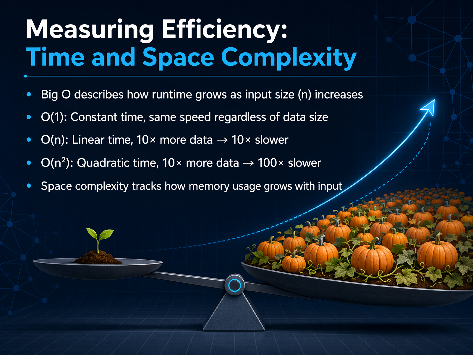
04Measuring Efficiency: Time and Space ComplexityNow let's talk about measuring efficiency. When we analyze an algorithm, we care about two things: how much time it takes and how much memory it uses. Big O notation is our way to describe this. It tells us how the runtime or the memory usage grows as the input size, which we call n, gets larger. We focus on the growth trend, not the exact number of seconds. Think of it like this: if you have ten times more data, does your code take ten times longer? A hundred times longer? Or does it not change at all? That's what Big O answers. For example, O of 1, or constant time, means the operation is lightning fast and stays that way no matter how big your data gets. Accessing an array element by its index is a perfect example. O of n, or linear time, means the time grows directly with the input. A simple loop that checks every item in a list is O of n. If you have ten times the data, it takes roughly ten times as long. O of n squared, or quadratic time, is a warning sign. This often happens with nested loops. If you have ten times the data, it can take a hundred times longer. And we can't forget space complexity. It tracks how much extra memory your algorithm needs as the input grows. Just like a recipe, you need to know how much counter space you'll need before you start cooking. Up next, we'll see these growth rates in action with some common examples.nedbatchelder.com blog.nadim.in geeksforgeeks.org+22 min
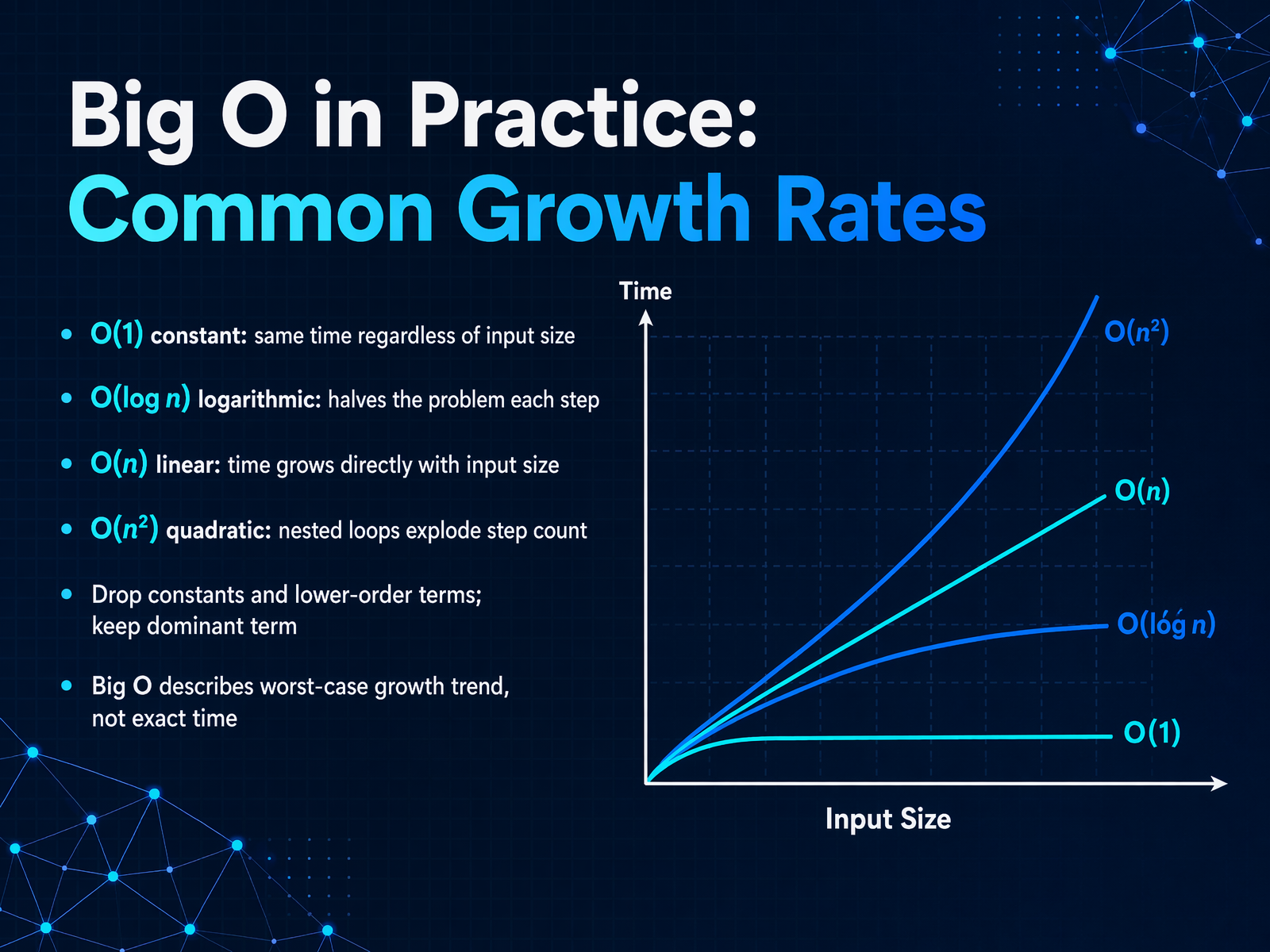
05Big O in Practice: Common Growth RatesNow let's make Big O practical and look at the common growth rates you will see in your own code. Think of these as the different speeds at which your algorithm can slow down as you feed it more data. First, O of one, or constant time. This is the ideal. It means your code takes the same number of steps regardless of input size. Accessing an array element by its index is a perfect example. Next, O of log n, or logarithmic time. This is highly efficient. The algorithm cuts the problem in half with every step, like a binary search. Doubling the data adds just one more step. Then we have O of n, or linear time. Time grows directly with the input size. A simple loop that visits every element once is linear. If you double the data, the time doubles. After that is O of n squared, or quadratic time. This is where you need to be careful. It usually means nested loops, where each loop depends on n. If you have a thousand items, you might end up with a million operations. The step count explodes. When you are analyzing your code, remember two key rules. First, drop the constants and lower-order terms. Keep only the dominant term that grows the fastest. Second, Big O describes the worst-case growth trend, not the exact number of seconds. It tells you how the algorithm will scale under pressure. Let's apply this scaling mindset to our next topic, searching, where we'll compare linear and binary search.nedbatchelder.com blog.nadim.in geeksforgeeks.org+22 min
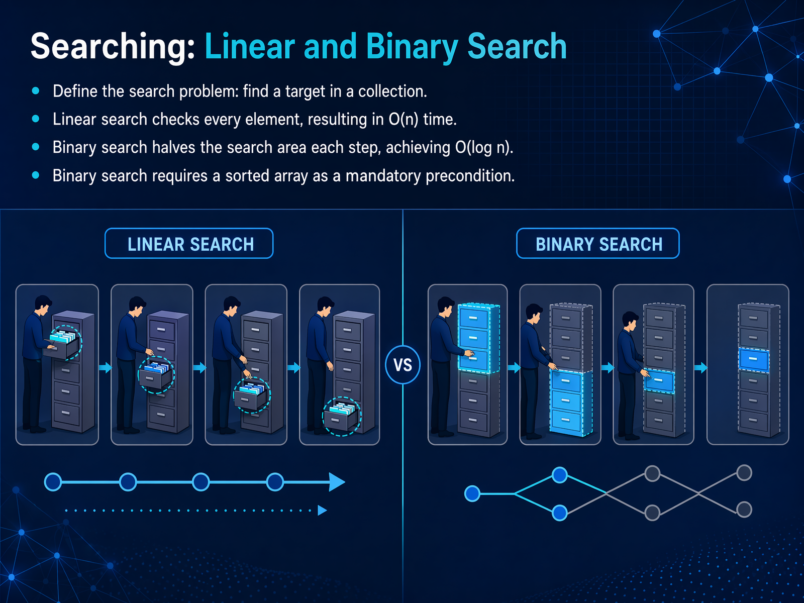
06Searching: Linear and Binary SearchNow let's turn to the classic search problem: finding a specific target inside a collection. Imagine you have a row of numbered lockers, and you need to find the one that contains a particular item. In computing, we have two main strategies for this. The first is linear search, where you simply start at the beginning and check every single locker until you find the target. This works on any list, but in the worst case, you might have to open every locker. We measure that cost as O of n. The second strategy is binary search, which is far more efficient. Think of how you look up a word in a physical dictionary. You don't start at page one and flip through every page. You open the book roughly in the middle, see which half your word falls into, and immediately discard the other half. Binary search does exactly this. It repeatedly checks the middle element, and if the target is smaller, it searches the left half; if larger, it searches the right half. Each comparison cuts the remaining search area in half, which gives us a logarithmic time complexity, O of log n. This is incredibly fast, even on millions of items. But there's a crucial precondition: the array must be sorted first. Without that sorted order, the halving logic simply doesn't work. Next, we'll walk through a step-by-step execution of binary search to see exactly how the pointers move and the search area shrinks.w3schools.com algo2vis.com coddy.tech+22 min
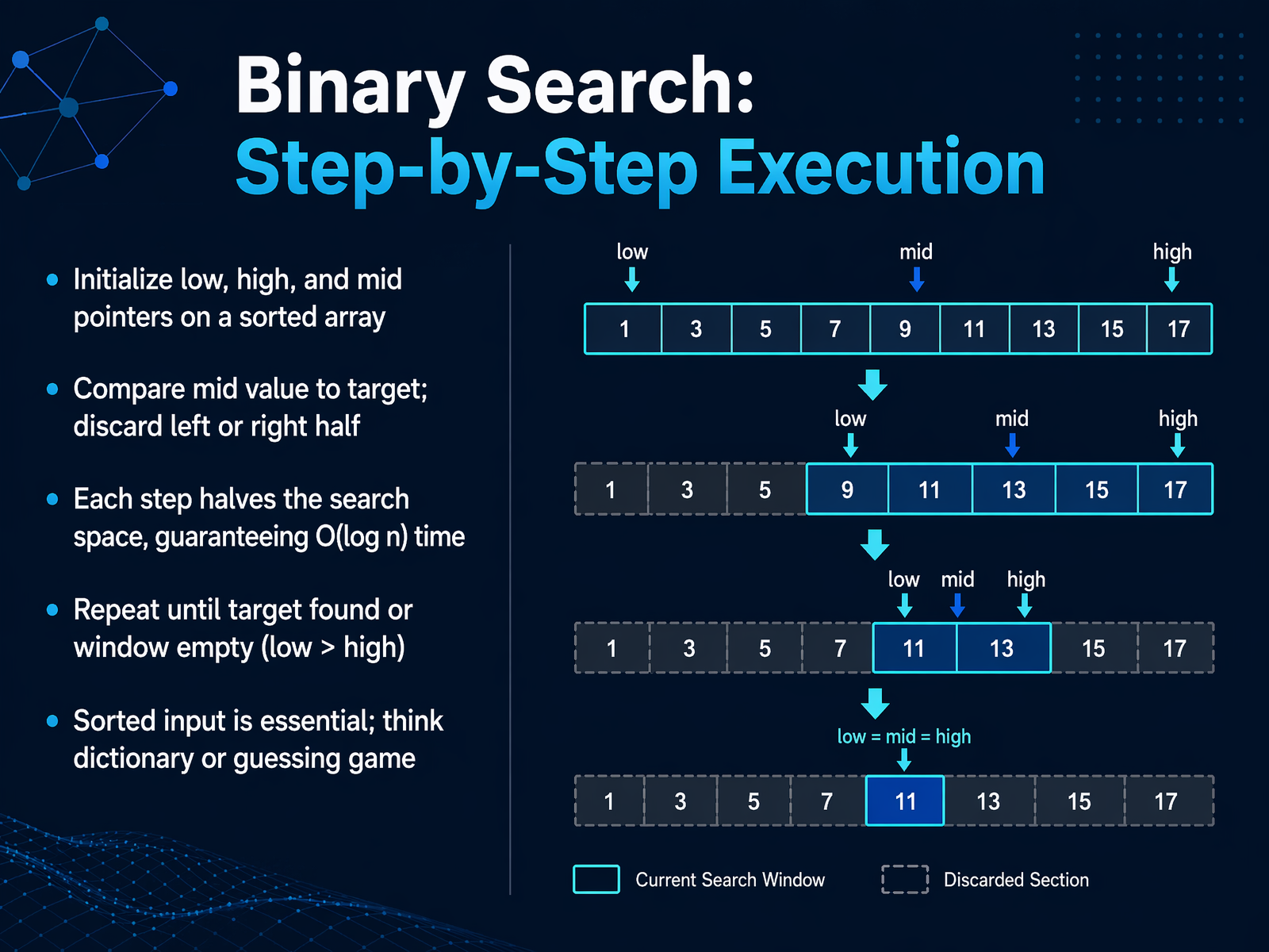
07Binary Search: Step-by-Step ExecutionNow, let's walk through exactly how binary search executes, step by step. The process always starts with three markers: we set a low pointer at the very first element, a high pointer at the last element, and then calculate the mid pointer right in the center. Think of it like opening a dictionary to the middle. You look at the word on that page. If your target word comes later alphabetically, you instantly discard the entire first half of the book. Binary search does the same thing. We compare the value at the mid pointer to our target. If the mid value is too small, we move the low pointer to mid plus one, throwing away the left half. If the mid value is too large, we move the high pointer to mid minus one, throwing away the right half. Each single comparison cuts the remaining search area exactly in half. That is why we guarantee a logarithmic, or O of log n, time complexity. We just repeat this halving process until we either find the target, or the low pointer crosses the high pointer, which means the window is empty and the target is not there. The one absolute requirement is that the input array must be sorted. Without sorted order, this whole halving logic breaks down. Next, we will explore sorting itself and why order matters so fundamentally.w3schools.com algo2vis.com coddy.tech+21 min
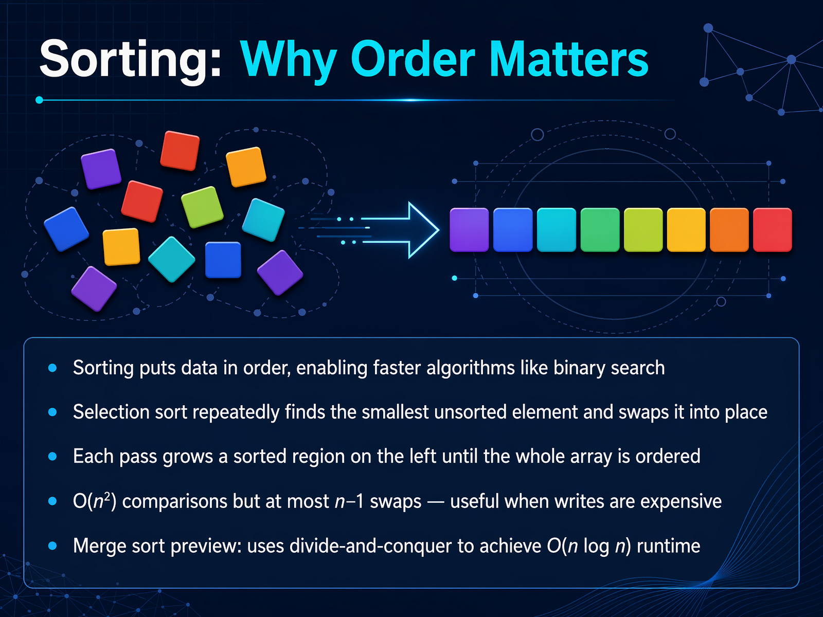
08Sorting: Why Order MattersNow let's look at a classic sorting method, selection sort, to see why ordering data matters. Imagine you have a row of unsorted numbers. Selection sort repeatedly scans that row to find the smallest remaining value, then swaps it into the correct position. Think of it like organizing a hand of playing cards by always picking the smallest card and moving it to the left. Each pass grows a sorted region on the left side. After the first pass, the smallest number sits at index zero. After the second pass, the next smallest sits at index one, and so on. The algorithm keeps shrinking the unsorted part until the whole collection is ordered. This approach always makes about n squared comparisons, but it performs at most n minus one swaps. That makes selection sort useful when writing data is expensive, like moving large records. 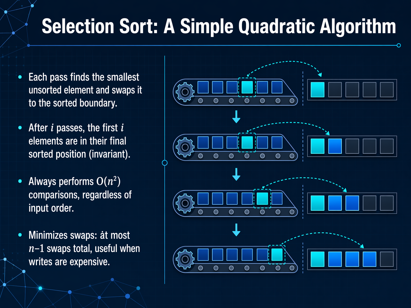Next, we'll explore selection sort in more detail, walking through its code and analyzing its quadratic runtime.1 min
09Selection Sort: A Simple Quadratic AlgorithmNow let's look at selection sort, a simple quadratic algorithm that's easy to understand and implement. Selection sort works by dividing the array into a sorted part on the left and an unsorted part on the right. On each pass, it scans the entire unsorted region to find the smallest element, then swaps that element into the first position of the unsorted region. That boundary then moves one step to the right, growing the sorted section. This gives us a powerful invariant: after i passes, the first i elements are in their final sorted position. They will never move again. Because it scans the entire unsorted tail every time, selection sort always performs O of n squared comparisons, even if the array is already sorted. However, it minimizes swaps. It performs at most n minus one swaps total, which makes it useful when writing to memory is expensive. For example, sorting an array of five elements requires at most four swaps. 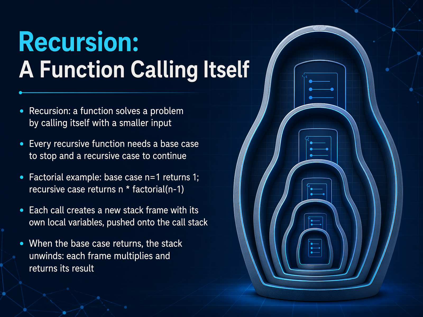Next, we'll explore a different approach: recursion, where a function calls itself.2 min
10Recursion: A Function Calling ItselfNow, let's explore one of the most powerful and initially mind-bending ideas in programming: recursion. Simply put, recursion is when a function solves a problem by calling itself with a smaller or simpler input. Think of it like a set of Russian nesting dolls. To open the biggest doll, you open a slightly smaller one inside it, and you keep going until you reach the tiniest doll that can't be opened—that's your stopping point. Every recursive function needs two critical parts. First, a base case, which is the simple condition that stops the recursion, like our tiny doll. Second, a recursive case, where the function calls itself, moving toward that base case. Let's make this concrete with a classic example: calculating a factorial. The factorial of a number n, written as n!, is n times n minus one, times n minus two, and so on, down to one. In a recursive function, the base case is when n equals one, and the function returns one. The recursive case is when n is greater than one, and the function returns n multiplied by the factorial of n minus one. So, what's actually happening under the hood? Each time the function calls itself, a new stack frame is pushed onto the call stack. This frame holds its own separate copy of the local variable n. The frames pile up until the base case is hit. Then, the stack unwinds: each frame returns its result to the one below it, multiplying the values as it goes, until the very first call produces the final answer. Understanding this stack mechanism turns recursion from magic into a predictable, traceable tool. 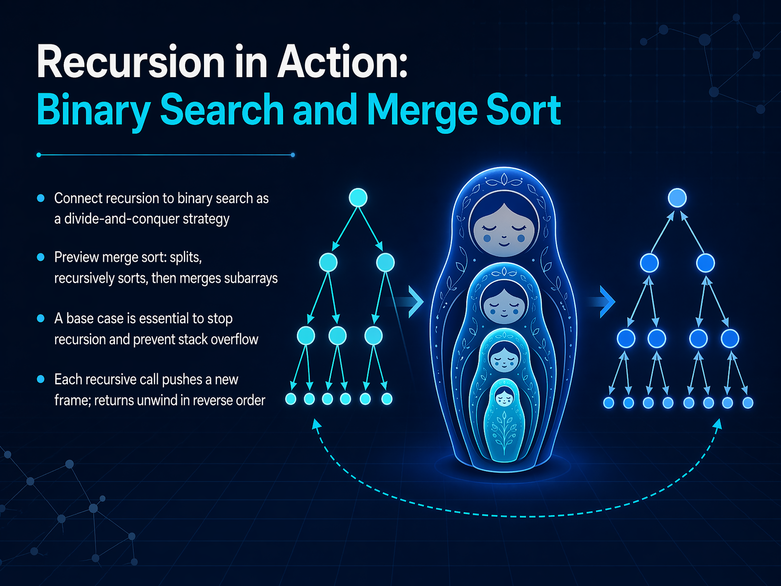Next, we'll see these concepts in action with more practical algorithms, starting with binary search and merge sort.2 min
11Recursion in Action: Binary Search and Merge SortNow let's see recursion in action with two powerful algorithms: binary search and merge sort. Both use a divide-and-conquer strategy — breaking a big problem into smaller, identical subproblems until the answer becomes obvious. Binary search works by repeatedly checking the middle element of a sorted array. If the target is smaller, it recursively searches the left half; if larger, the right half. Each call cuts the search space in half. Merge sort takes this further. It splits an array into two halves, recursively sorts each half, then merges the sorted halves back together. The key to making all of this work is the base case. Without a base case, the recursion never stops, and the call stack overflows. Speaking of the stack, remember that each recursive call pushes a new frame onto the call stack. Those frames hold the function's local variables and pause execution. Once the base case is reached, the frames unwind in reverse order, each returning its result to the caller below. So the deepest call finishes first, and the initial call finishes last. Understanding this push and unwind cycle is what makes recursion feel predictable instead of magical. 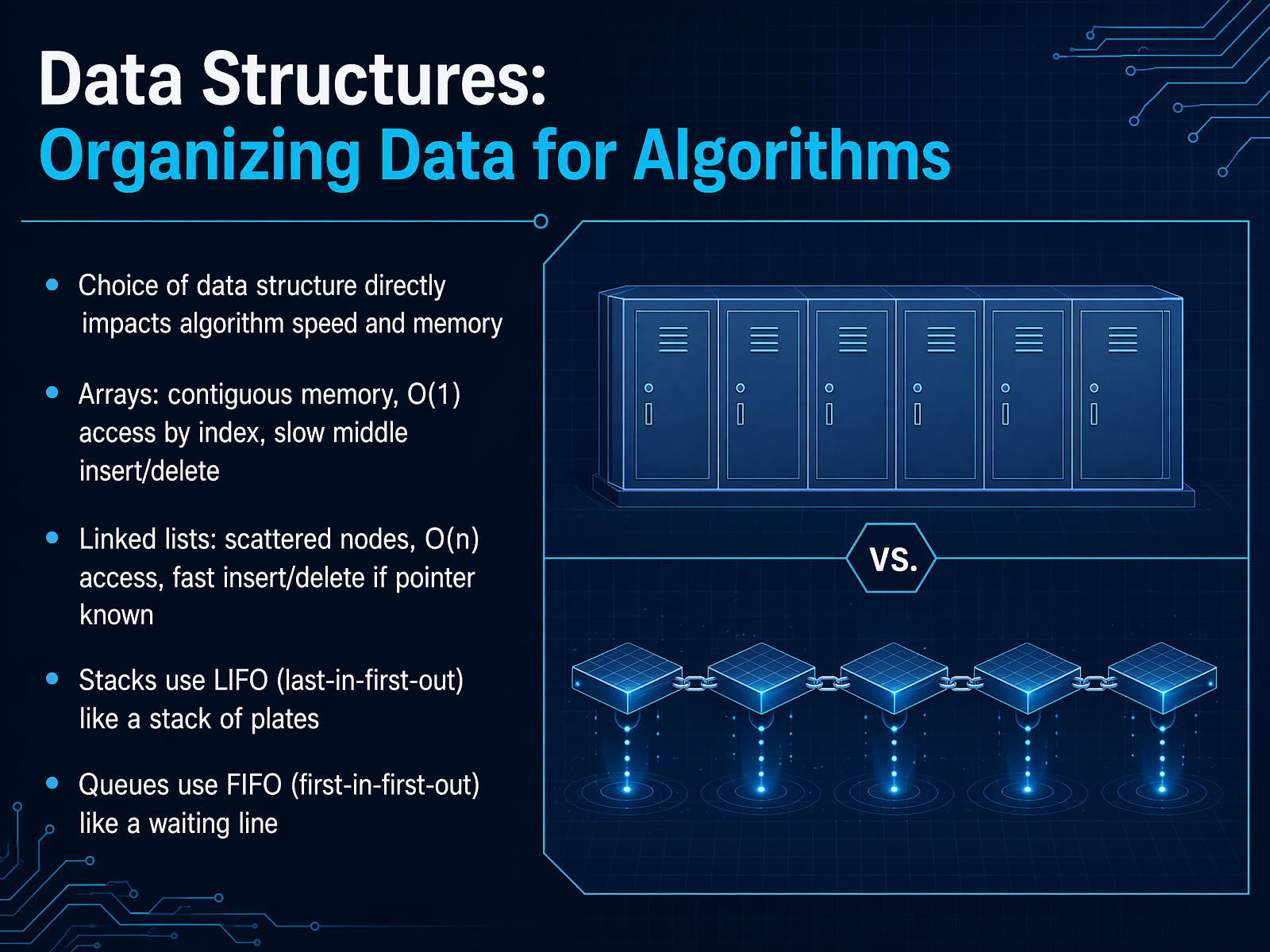Coming up next, we'll shift our focus to data structures and how they organize data for algorithms.2 min
12Data Structures: Organizing Data for AlgorithmsChoosing the right data structure is one of the most impactful decisions you'll make, because it directly controls your algorithm's speed and memory usage. Let's walk through four essential structures, starting with the array. An array stores elements in a single, contiguous block of memory. This layout gives you O of one, or constant-time, access to any element by its index. However, inserting or deleting an element in the middle is slow, an O of n operation, because the remaining elements must shift to fill the gap. Next, consider the linked list. Here, each element is a separate node in memory, connected by pointers. Access is slower because you must traverse from the head, taking O of n time. But if you already have a pointer to the insertion point, adding or removing a node is a fast, O of one pointer update. Two other structures give you strict rules for ordering. A stack operates on a last-in-first-out, or LIFO, principle, just like a stack of plates where you always take the top one. A queue, in contrast, uses a first-in-first-out, or FIFO, model, exactly like a waiting line where the first person to arrive is the first to be served. Your choice of structure shapes every operation that follows. 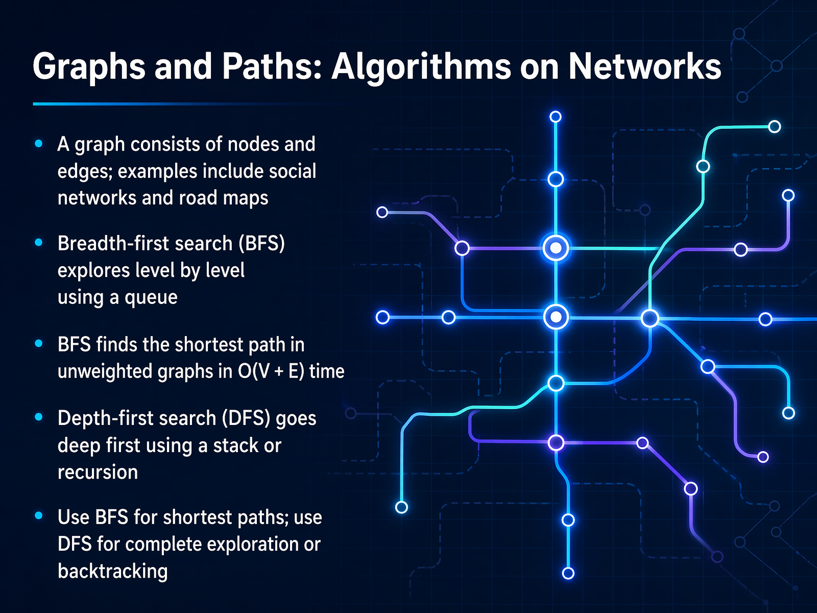Next, we'll move beyond simple sequences and explore graphs and paths, applying algorithms on networks.2 min
13Graphs and Paths: Algorithms on NetworksLet's move on to graphs and the paths that connect them. Think of a graph as a network. The nodes are people in a social network, and the edges are their friendships. Or, nodes are intersections on a map, and edges are the roads between them. When we need to find a route or a connection, we use traversal algorithms. The first one is breadth-first search, or BFS. BFS explores a graph level by level. It starts at a source node, visits all its immediate neighbors first, then visits their neighbors, and so on. To do this, it uses a queue to keep track of the order. Because BFS fans out evenly, it always finds the shortest path in an unweighted graph, measured by the fewest number of edges. Its time complexity is O of V plus E, where V is vertices and E is edges. The second algorithm is depth-first search, or DFS. DFS takes the opposite approach. It picks one path and goes as deep as possible before backtracking. It uses a stack or recursion to manage its exploration. Use BFS when you need the shortest path, like finding the quickest route on a map with equal distances. Use DFS when you need to explore every possible path completely, like solving a maze or checking all connected components. 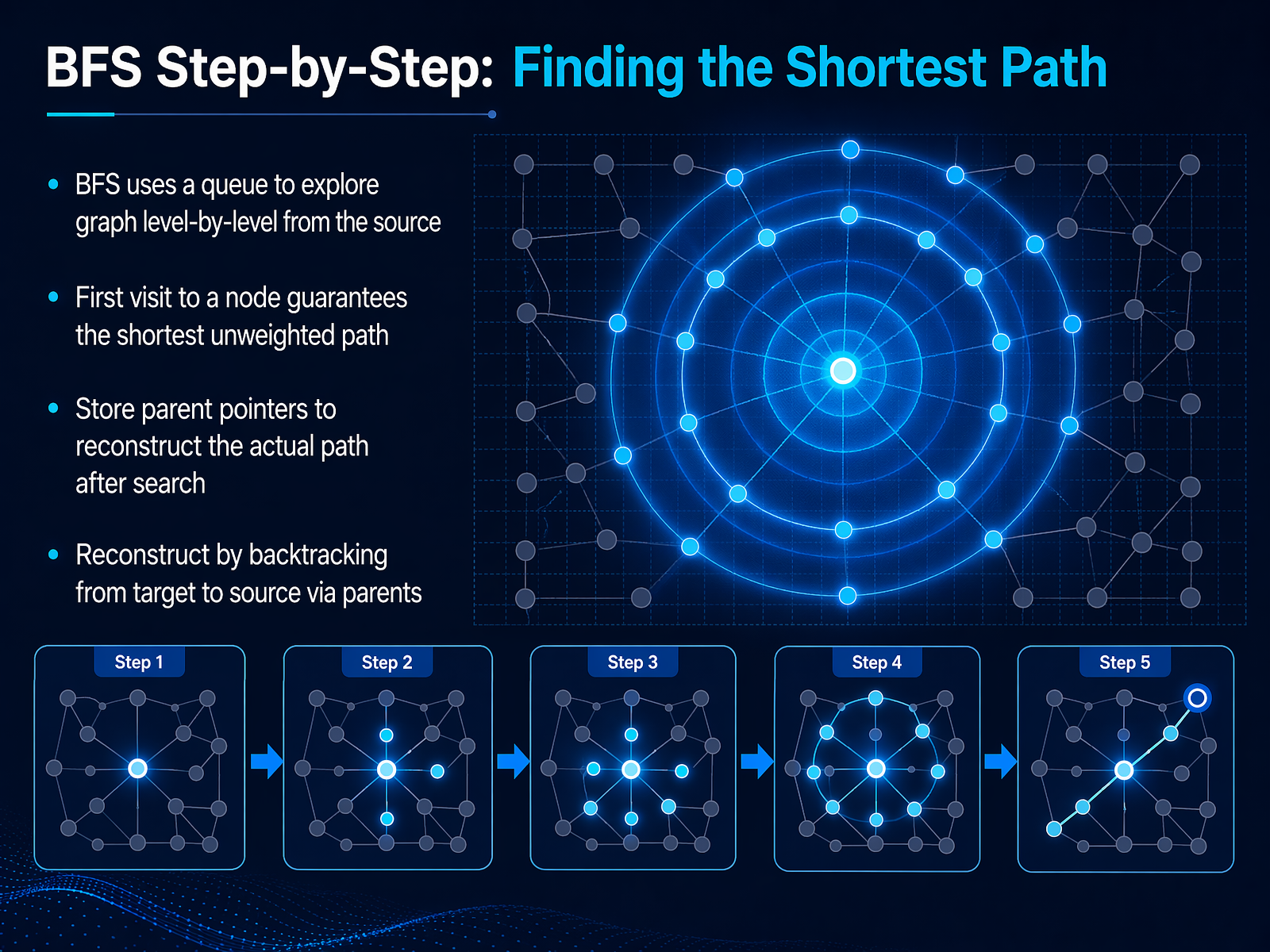Now, let's see BFS in action step by step to find the shortest path.2 min
14BFS Step-by-Step: Finding the Shortest PathNow let's walk through how BFS actually finds the shortest path, step by step. The key is that BFS uses a queue to explore the graph level by level, starting from the source node. Think of it like pouring water on a flat surface. It spreads out evenly in all directions, reaching the closest nodes first before moving further out. Because of this, the very first time we visit a node, we have found the shortest possible path in an unweighted graph. There is no faster way to get there. To actually retrieve that path, we store parent pointers, or predecessors, as we go. Each time we discover a new node, we record which node we came from. Then, once the search reaches the target, we can reconstruct the full path. We do this by backtracking from the target, following the chain of parent pointers all the way back to the source. This gives us the shortest path in reverse order, which we then flip to get the correct sequence. This simple backtracking mechanism is what turns a level-by-level exploration into a precise route planner. 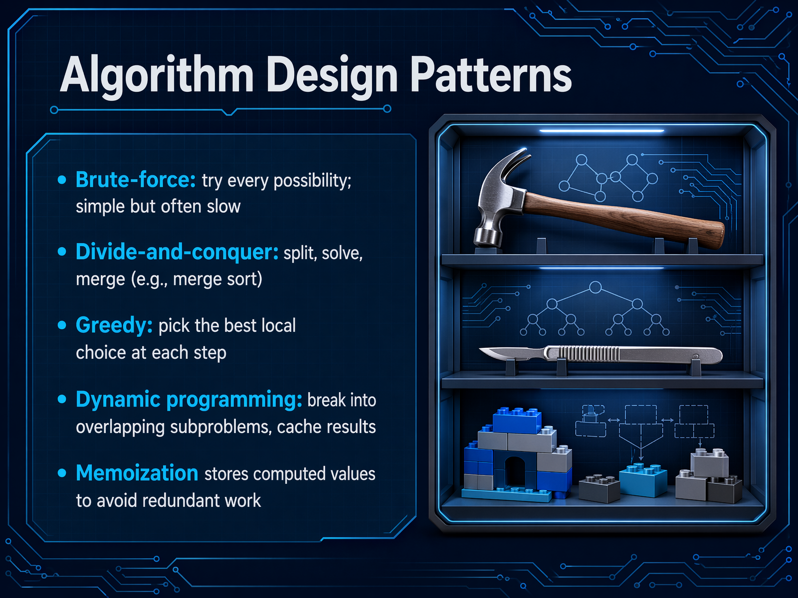Next, we will look at common algorithm design patterns that build on these fundamental traversal techniques.2 min
15Algorithm Design PatternsNow that we've seen some core algorithm concepts, let's step back and look at the common design patterns you'll use to build your own solutions. These are like blueprints for problem-solving. First, brute-force. This pattern tries every single possibility until it finds the answer. It's simple to write, but often very slow, so you use it for small inputs or as a starting point. Next, divide-and-conquer. You break the problem into smaller, independent pieces, solve them, and then merge the results. Merge sort is a classic example. Third, greedy algorithms. At each step, you pick the choice that looks best right now. It's fast, but it doesn't always give the perfect answer. You have to be sure the problem fits. Finally, dynamic programming and memoization. These work when a problem has overlapping subproblems—like calculating Fibonacci numbers. In a naive recursion, you recompute the same values over and over. Memoization fixes that. It simply stores the result of each calculation in a cache. The next time you need it, you just look it up instead of recalculating, turning an exponential-time problem into a linear one. For example, finding the thirtieth Fibonacci number without memoization takes over two million computations. With it, you need just thirty-one. That's the power of trading a little memory for a huge speed boost. 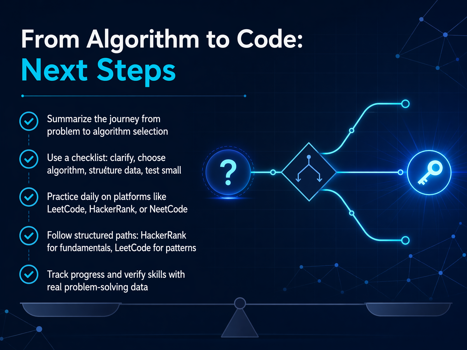Next, we'll wrap up by looking at how to move from an algorithm on paper to actual code.2 min
16From Algorithm to Code: Next StepsAnd here we are at the final step of our journey. You have moved from a vague problem to a clear algorithm, structured your data, and tested your logic on a small scale. Now, let's turn that understanding into a sustainable habit. Start by using a simple checklist before you write any code. First, clarify the problem completely. Second, choose the algorithm that fits. Third, structure your data properly. And fourth, test your logic with a tiny example. This checklist keeps you grounded and prevents you from jumping straight into code without a plan. To build this skill, practice daily. Platforms like HackerRank are perfect for building fundamentals, while LeetCode helps you recognize common patterns. For structured, beginner-friendly roadmaps, check out NeetCode, which offers video explanations and clear learning paths. As you solve problems, track your progress. Your acceptance rate, consistency, and growing speed are real data points that verify your skills. They prove you are not just memorizing solutions, but truly mastering the logic. Thank you for taking this first step into structured problem-solving. Keep your checklist handy, stay curious, and enjoy the satisfaction of watching your code work exactly as planned. Happy coding.2 min

Sources consulted

Web sources consulted while building this course.