Descriptive Statistics: Concepts and Applications

What you’ll learn

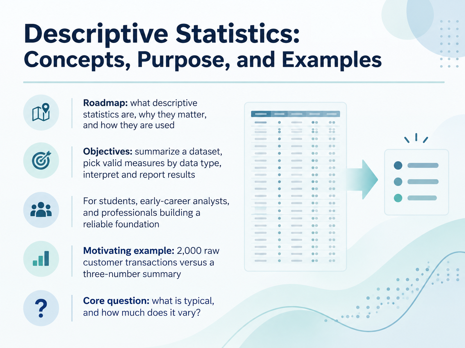
1. 01Descriptive Statistics: Concepts, Purpose, and ExamplesWelcome. I'm glad you're here. This course builds a reliable foundation in descriptive statistics, whether you're a student, an early-career analyst, or a professional brushing up on the basics. Here's our roadmap. First, we'll define what descriptive statistics are. Next, we'll see why they matter. Then, we'll practice using them by data type. Our objectives are practical. You'll learn to summarize a dataset, choose valid measures for the data you have, and interpret and report results clearly. Consider a motivating example. Imagine two thousand raw customer transactions. Scanned line by line, they tell you very little. Summarized into three numbers, such as the typical purchase amount, the spread around it, and the most common count, they tell a story. That leads to our core question: what is typical, and how much does it vary? Keep that question in mind. Now, let's look at what descriptive statistics are and are not.dictionary.apa.orginvestopedia.commathworld.wolfram.com+22 min
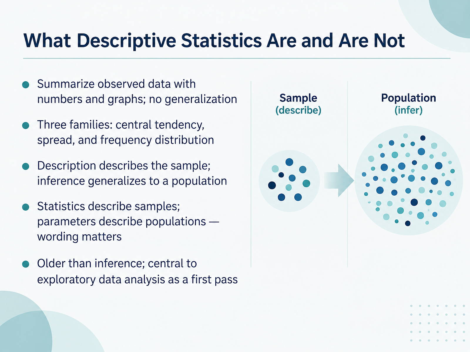
2. 02What Descriptive Statistics Are and Are NotNow let's define our tool. Descriptive statistics summarize data you actually observed, using numbers and graphs. They do not generalize beyond that data. Think of them as three families: central tendency, like a mean; spread, like a range; and frequency distribution, like a histogram. Here is a common confusion. Descriptive statistics describe the sample. Inferential statistics generalize to a population. Related to that, statistics describe samples, and parameters describe populations. Wording matters. Descriptive methods are older than inference. They are central to exploratory data analysis, your first pass before testing ideas. Quick takeaway: use description to understand what you have, and save inference for later. Next, let's look at why bothering to summarize data pays off.2 min
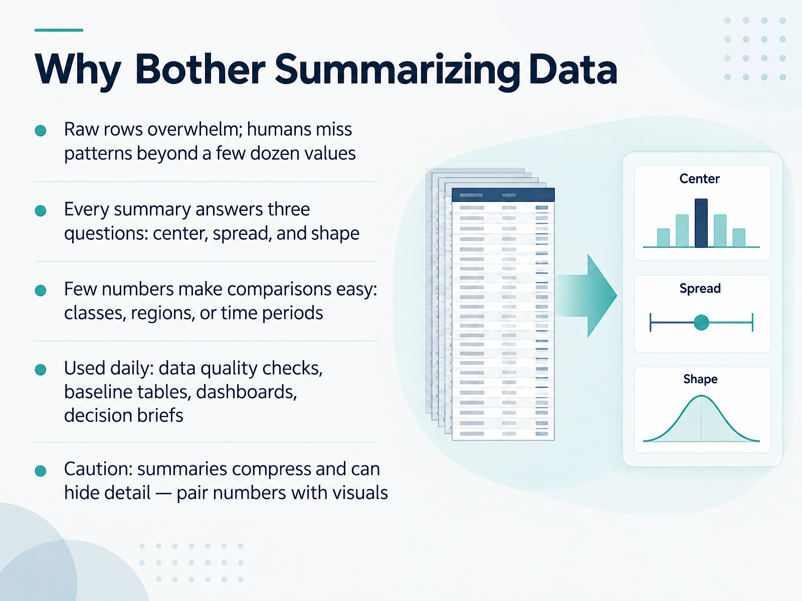
3. 03Why Bother Summarizing DataNow let's talk about why summarizing data is worth your time. First, picture a spreadsheet with thousands of raw rows. Beyond a few dozen values, humans simply can't spot patterns by eye. Summaries solve that. Every summary answers three questions: center, meaning the typical value, spread, meaning how much values vary, and shape, meaning how the values are distributed. Here's why it matters: a few numbers make comparisons easy, whether you're comparing classes, regions, or time periods. You'll use summaries daily, in data quality checks, baseline tables, dashboards, and decision briefs. But a caution. Summaries compress information, so they can hide important detail. Always pair summary numbers with visuals. Your takeaway is this: summarize to see patterns, then check the details. Next, we'll look at data types and measurement scales.2 min
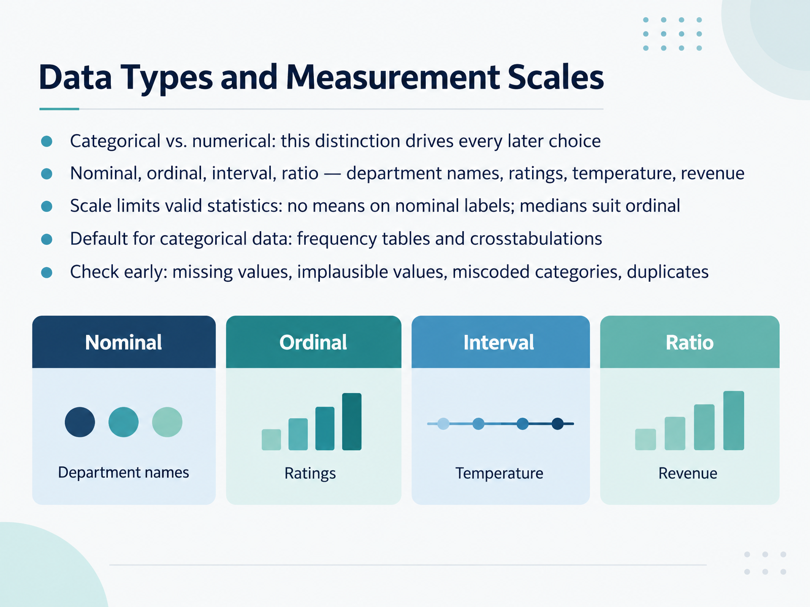
4. 04Data Types and Measurement ScalesNow let's look at data types and measurement scales. First, data splits into categorical and numerical, and this distinction drives every later choice you make. Categorical data labels groups, like department names on an ordinal scale of ratings, while numerical data measures quantities, like temperature or revenue on interval and ratio scales. Next, the scale limits which statistics are valid. You cannot take a mean of nominal labels, and medians suit ordinal ratings. Here's why it matters: the right scale protects your conclusions. For categorical data, the default is frequency tables and crosstabulations. Check early for missing values, implausible values, miscoded categories, and duplicates. Your takeaway: confirm your data types and scales before analyzing. Next, we move to measures of central tendency.1 min
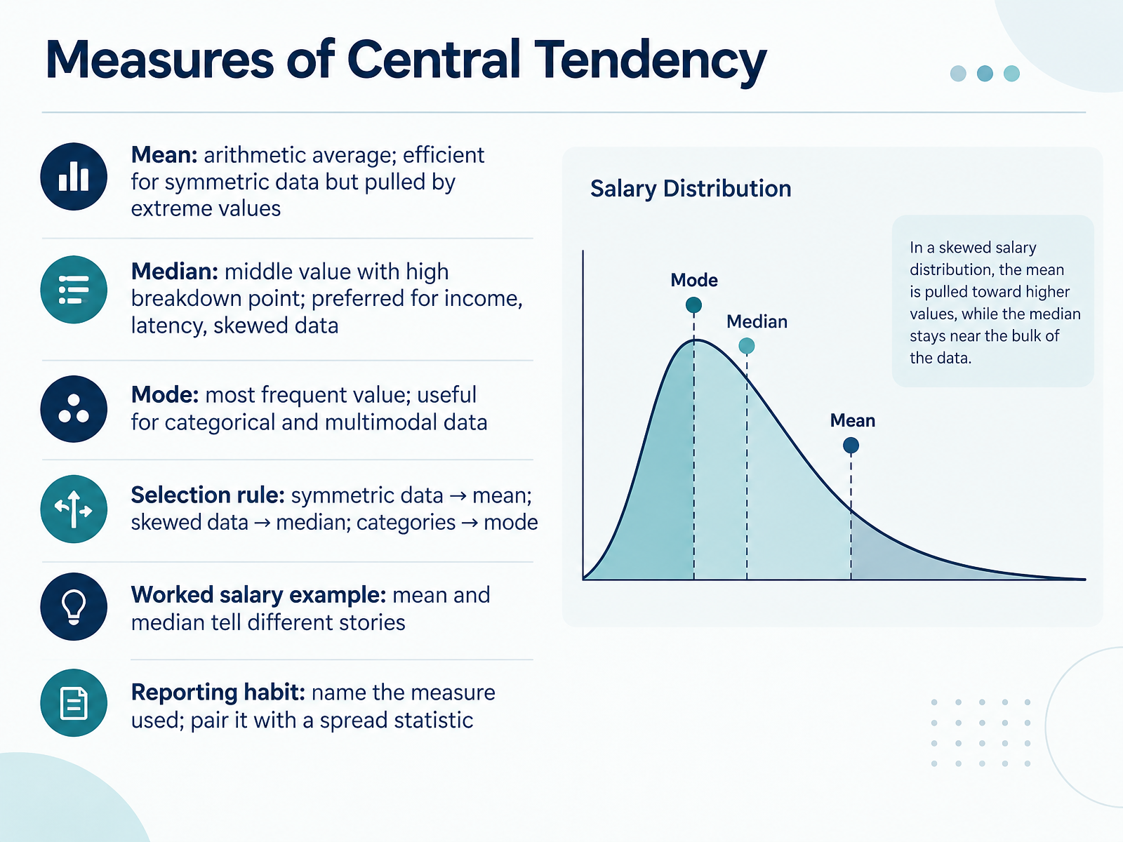
5. 05Measures of Central TendencyNext, let's look at measures of central tendency, which summarize a dataset with one typical value. The mean is the arithmetic average. It's efficient for symmetric data, but extreme values can pull it. The median is the middle value when data is ordered. It has a high breakdown point, so it's preferred for income, latency, and skewed data. The mode is the most frequent value, useful for categories and multimodal data. Here's the selection rule. Symmetric data points to the mean. Skewed data points to the median. Categories point to the mode. Consider salaries. If most people earn forty thousand and one executive earns four hundred thousand, the mean jumps high, while the median stays near forty thousand. Both are correct, but they tell different stories. So name the measure you used, and pair it with a spread statistic. Coming up next, Measures of Spread and Variability.1 min
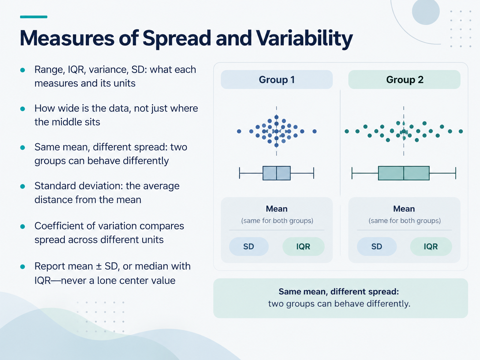
6. 06Measures of Spread and VariabilityNow let's move from the center of your data to its spread. Two groups can share the same mean yet behave very differently, which is why you also need to know how wide the data is. The range is the highest value minus the lowest, and it uses your data's units. The interquartile range, or IQR, covers the middle fifty percent of values, also in your units. Variance measures average squared distance from the mean, so its units are squared. Standard deviation is the square root of variance, which brings you back to your original units. Think of it as the average distance from the mean. When units differ, the coefficient of variation, standard deviation divided by the mean, lets you compare spread fairly. In practice, report mean plus or minus standard deviation, or median with IQR, never a lone center value. Next, we'll look at distribution shape, skewness, and outliers.2 min
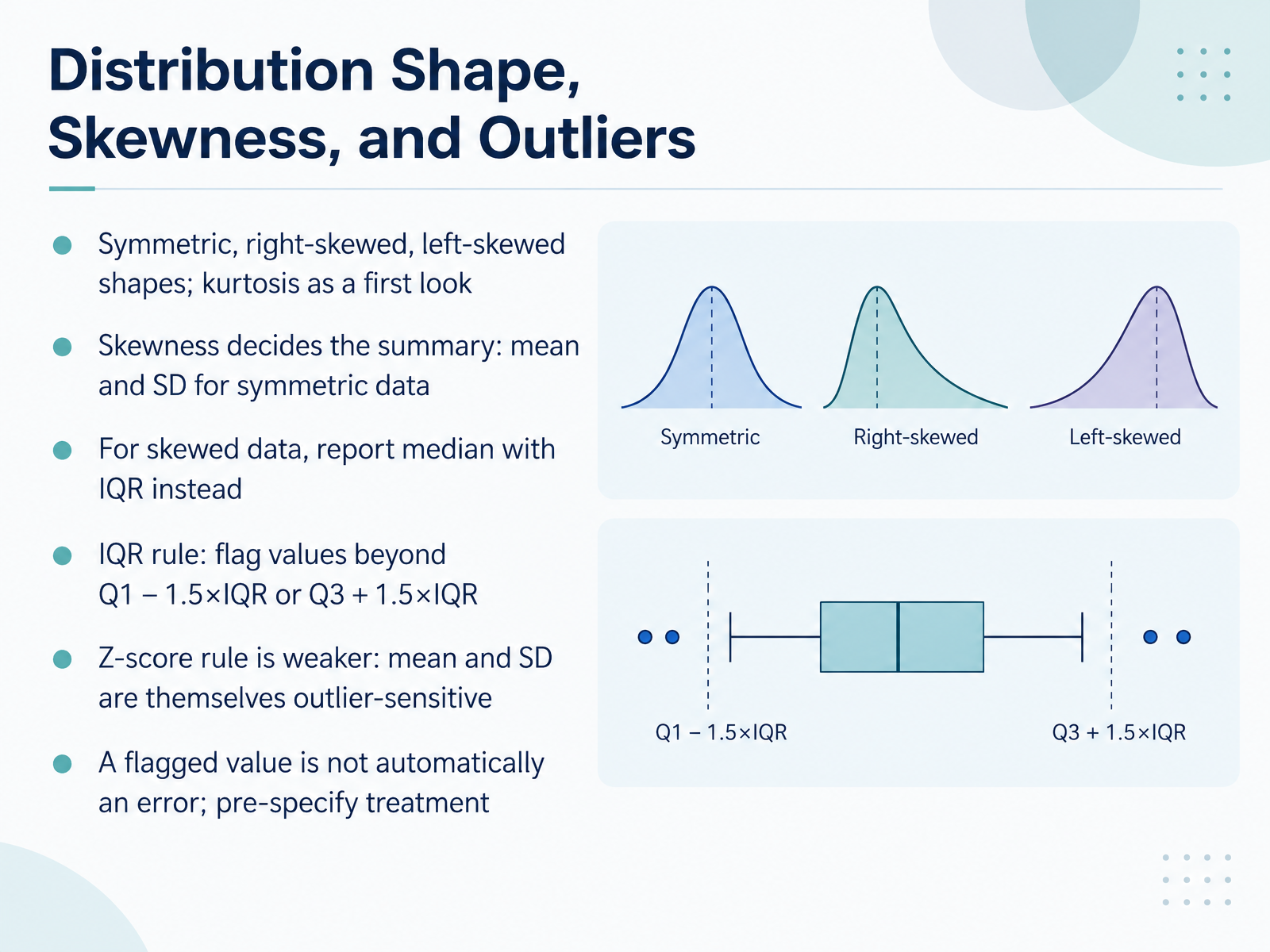
7. 07Distribution Shape, Skewness, and OutliersNext, let's look at the shape of your data. A distribution can be symmetric, right-skewed, or left-skewed, and kurtosis gives you a first look at how heavy its tails are. Here's why it matters. Skewness decides which summary you report. For symmetric data, report the mean and standard deviation. But for skewed data, use the median with the interquartile range, or IQR. To flag outliers with the IQR rule, mark any value below Q1 minus one point five times the IQR, or above Q3 plus one point five times the IQR. You may also hear about the z-score rule, but it is weaker, because the mean and standard deviation are themselves sensitive to outliers. Finally, remember that a flagged value is not automatically an error. Decide how you will treat outliers before you analyze, and document that choice. Next, we will see these ideas in action in Visualizing Descriptive Statistics.2 min
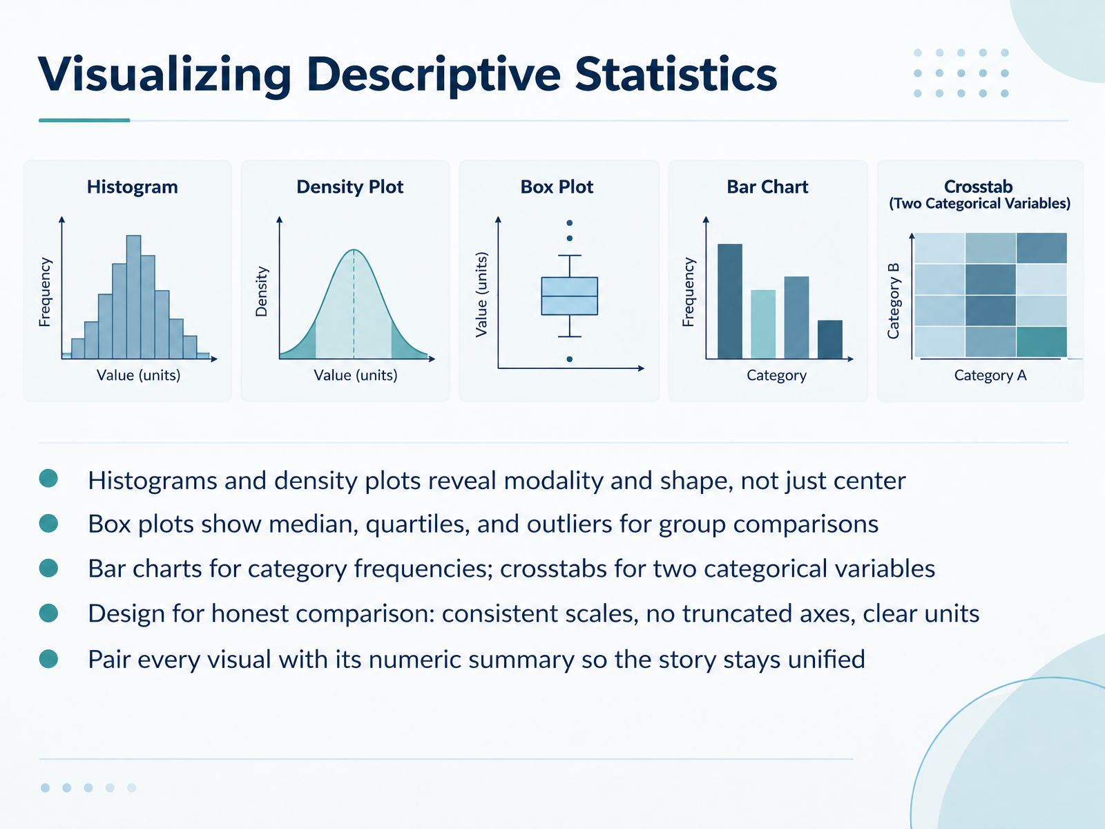
8. 08Visualizing Descriptive StatisticsNext, let's look at how we visualize descriptive statistics, because the right picture makes patterns easier to see. Start with histograms and density plots. A histogram groups values into bins and shows how often each range occurs. It reveals modality, meaning how many peaks the data has, and shape, like skew, not just the center. Next, box plots show the median, the quartiles, and outliers, which makes them useful for comparing groups side by side. For categories, use bar charts to show category frequencies, and crosstabs when you have two categorical variables and want to see how they combine. Here's why design matters. Keep scales consistent, avoid truncated axes, and label units clearly, so comparisons stay honest. Finally, pair every visual with its numeric summary, such as the mean and median, so the story stays unified. A quick takeaway: choose the visual that answers your question, then check it against the numbers. That leads us into a practical workflow with a worked example.1 min
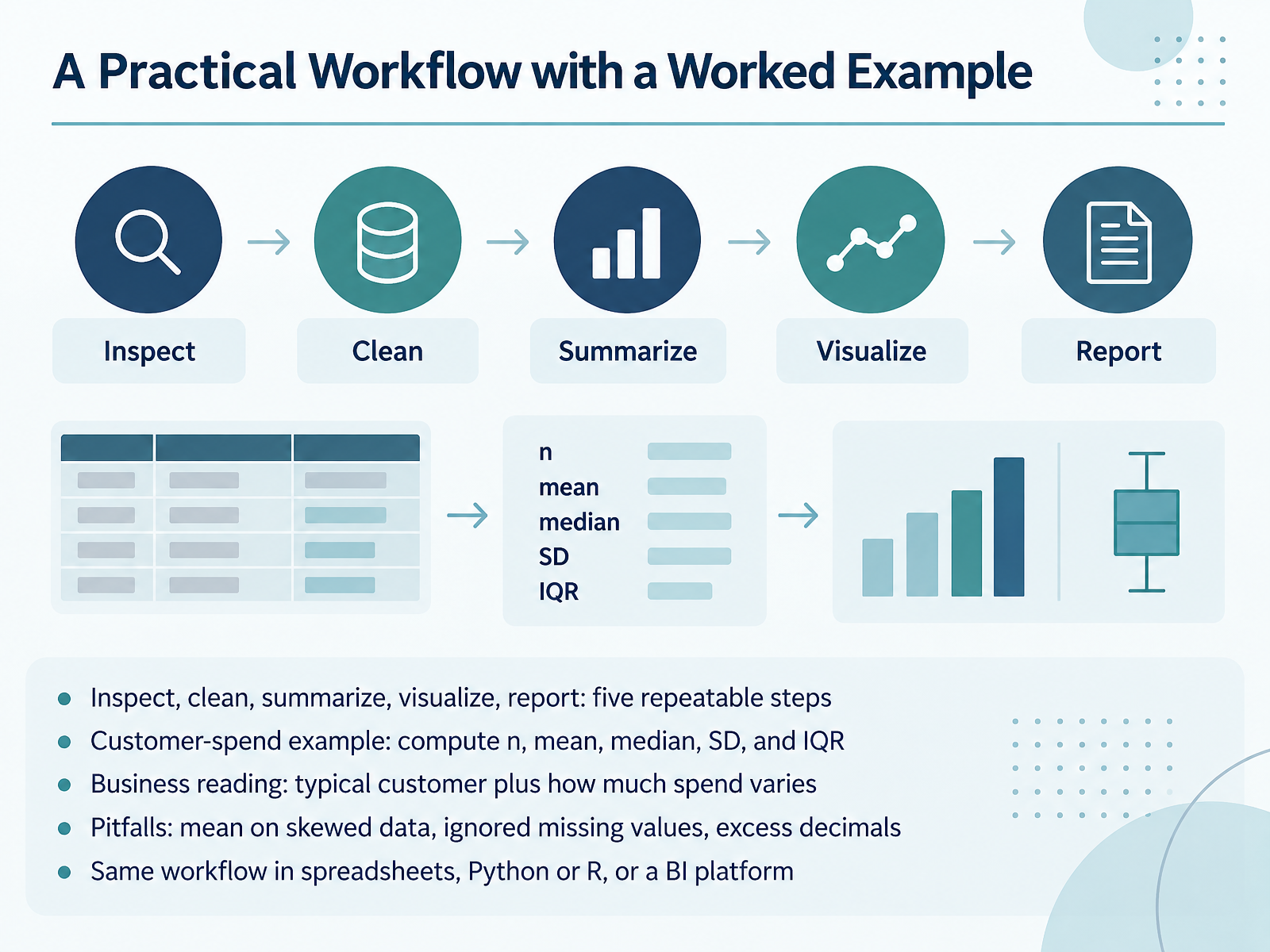
9. 09A Practical Workflow with a Worked ExampleNow let's put everything together into a practical workflow. First, inspect your data. Then clean it. Next, summarize it. After that, visualize it. And finally, report it. These five steps repeat every time, and they keep your analysis reliable. Here's a worked example with customer spend. Compute n, the count of customers. Then the mean and the median. Then the standard deviation and the interquartile range. The business reading is simple: the median tells you what a typical customer spends, and the spread measures tell you how much spending varies. Watch for three common pitfalls. Don't use the mean on skewed data. Don't ignore missing values. And avoid excess decimals in your report. You can run this same workflow in spreadsheets, in Python or R, or in a business intelligence platform. Your takeaway is this: follow the five steps every time, and your results stay consistent and trustworthy. Next, we'll look at reporting descriptive results correctly.2 min
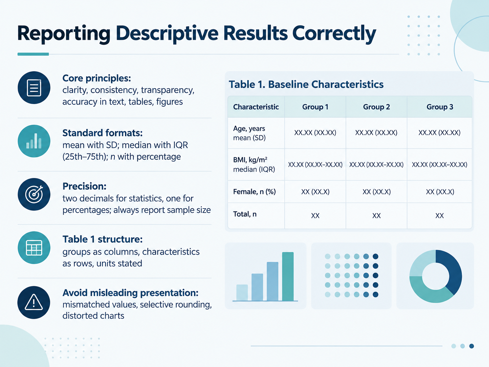
10. 10Reporting Descriptive Results CorrectlyNow let's turn to reporting descriptive results correctly. The core principles are clarity, consistency, transparency, and accuracy across your text, tables, and figures. For standard formats, report the mean with the standard deviation, or the median with the interquartile range, shown as the twenty-fifth to seventy-fifth percentile. For counts, use n with a percentage. On precision, use two decimals for statistics and one for percentages, and always report the sample size. In a Table One, put groups as columns, characteristics as rows, and state units. Avoid mismatched values, selective rounding, and distorted charts. Here's your takeaway: check every table against these rules before you share it. Next, we look at matching the summary to the audience and decision.1 min
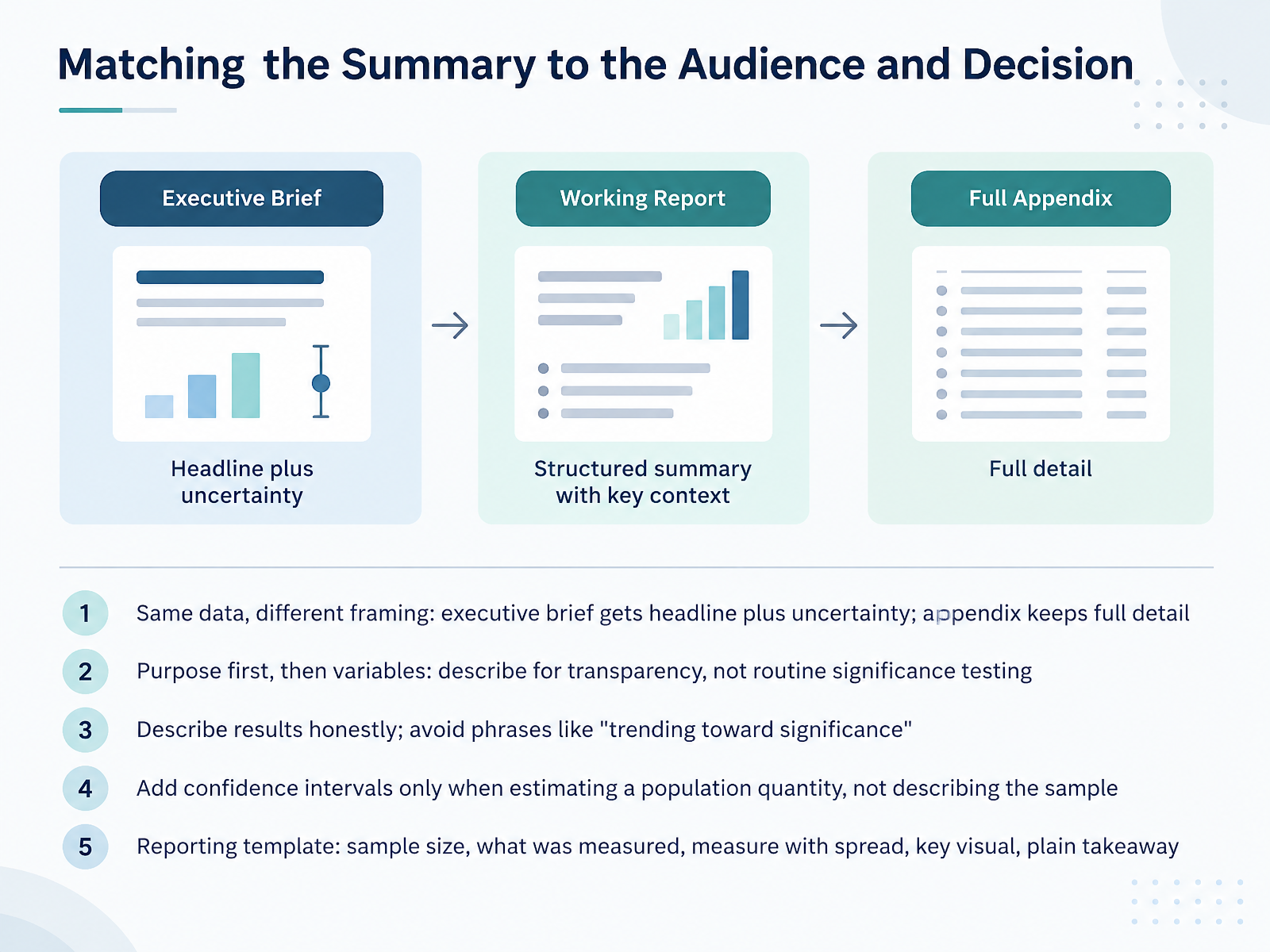
11. 11Matching the Summary to the Audience and DecisionNow let's talk about matching your summary to the audience and the decision. The same data can be framed differently. An executive brief gets the headline plus uncertainty, while an appendix keeps the full detail. Start with purpose, then choose variables. Describe for transparency, not routine significance testing. Be honest in your results. Avoid phrases like trending toward significance, because they overstate what the data show. Add confidence intervals only when you are estimating a population quantity, not when you are simply describing the sample. Here is a practical reporting template. State the sample size, what was measured, the measure with its spread, one key visual, and a plain takeaway. Next, we will apply these choices in a guided practice on selecting measures for a dataset.2 min
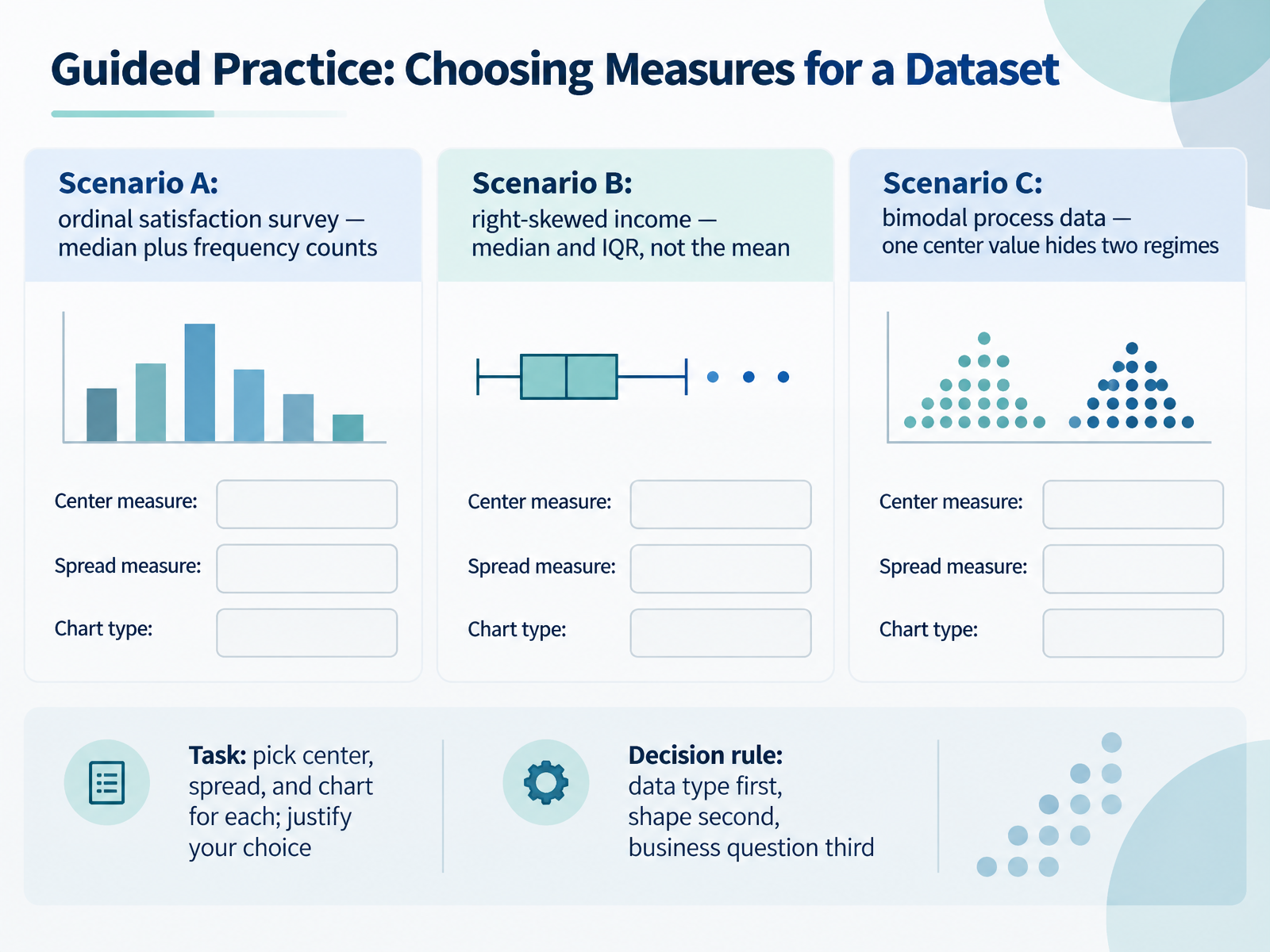
12. 12Guided Practice: Choosing Measures for a DatasetNow let's practice choosing measures together. Here are three scenarios, and your task is to pick a center, a spread, and a chart for each, then justify your choice. First, Scenario A: an ordinal satisfaction survey. The data are ordered categories, so use the median plus frequency counts. Next, Scenario B: right-skewed income. A few high earners pull the mean upward, so report the median and the interquartile range, not the mean. Then, Scenario C: bimodal process data. A single center value hides two regimes, so look at the shape before you summarize. Use this decision rule: data type first, shape second, business question third. Take a moment to write your choices, then explain them to a colleague. That justification is where real understanding shows. Next, we'll interpret and critique descriptive output.2 min
13. 13Guided Practice: Interpreting and Critiquing Descriptive OutputNow let's put these ideas into practice with a short guided critique. First, read the summary table and state the typical case and variability in one sentence, for example: the median order value is forty-two dollars, with an interquartile range of eighteen dollars. Next, spot common errors. A mean reported on skewed data, a missing sample size, or inconsistent decimal places should all raise a flag. Then judge the outlier decision. Was the rule specified before analysis, and is the effect of excluding outliers disclosed? After that, critique the charts. Check for a truncated axis, missing units, and visuals that contradict the numbers. Finally, apply a peer-review checklist drawn from reporting guidelines, and use it on the next report you read. In the final section, we'll pull together the key takeaways and next steps.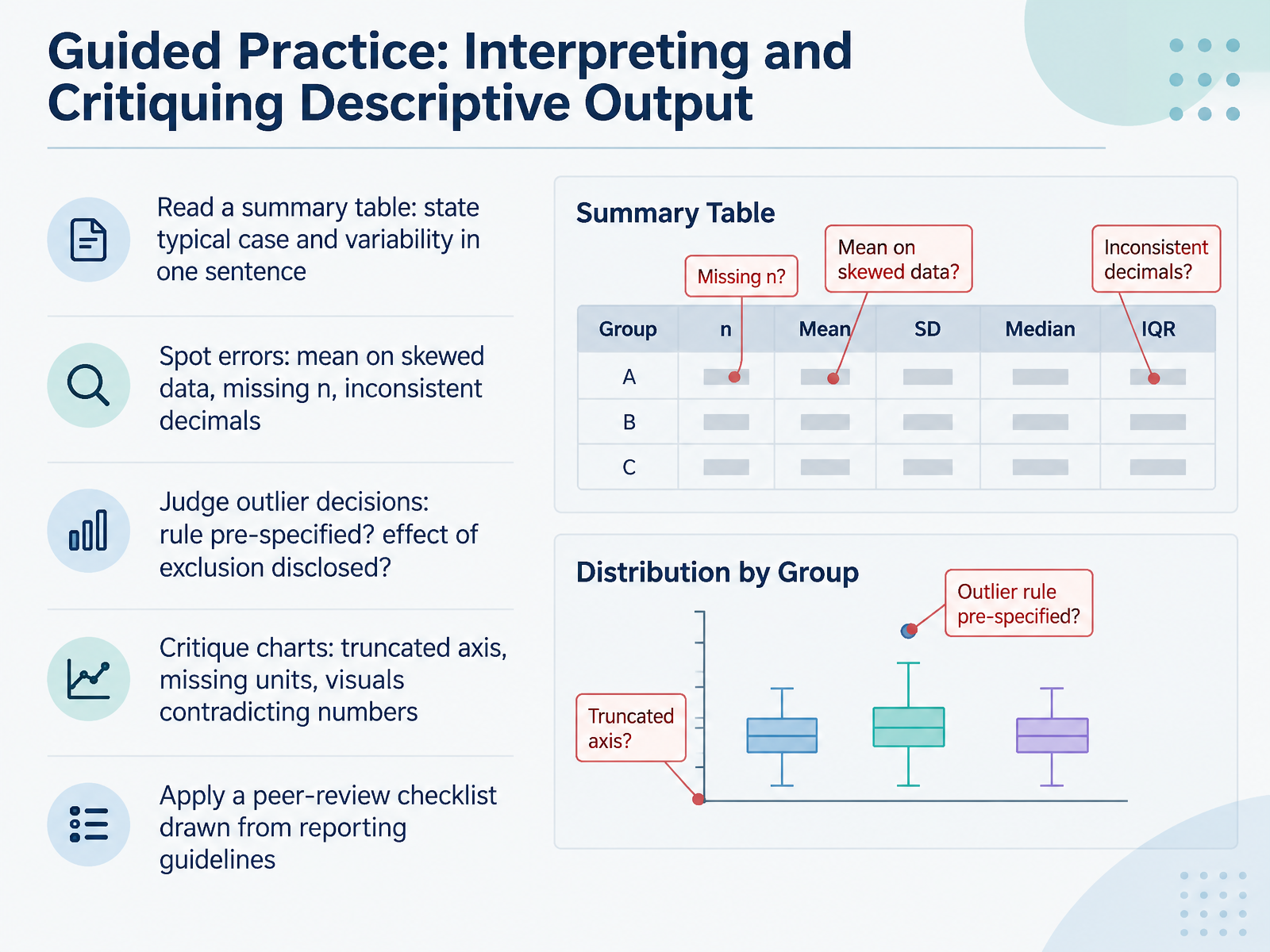2 min
14. 14Key Takeaways and Next StepsLet's bring it all together. First, descriptive statistics summarize three things about observed data: center, spread, and shape. Next, the type and shape of your data dictate which measure to use, and you should always report center, spread, and n together. For example, a median of forty dollars means little without the spread and the sample size beside it. Pair visuals with numbers, and decide how you'll handle outliers before you analyze, not after. Here's why that matters: pre-specified choices keep your results honest and reproducible. From here, inferential statistics is your next step, where confidence intervals and tests build directly on these summaries. So try it yourself: run the five-step workflow on a small dataset of your own. You now have a practical foundation, so thank you for learning with me, and keep practicing with confidence.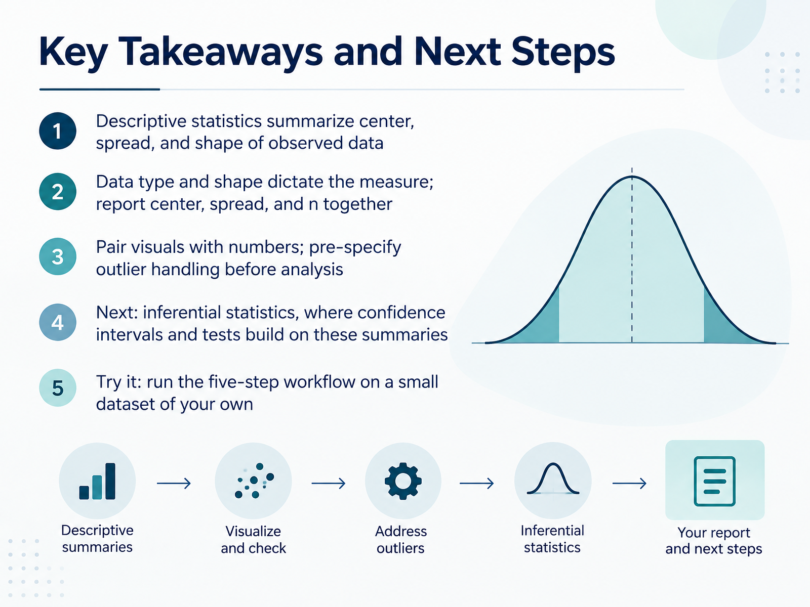1 min

Take the deck with you

Download this course as a file — free, no sign-up needed.

• PDF handoutEvery slide page, ready to print or share.15 pages · 2.9 MBDownload
• Narrated PowerPointThe deck that presents itself — every slide carries the digital human's narration video.15 pages · 12.4 MBDownload
• PowerPoint slidesThe full deck as a .pptx — open it in PowerPoint, Keynote, or Google Slides.15 pages · 2.8 MBDownload

Free to use in your own training — please keep the PersonWise credit page at the end.

Have your own deck? Turn it into a course

Sources consulted

Web sources consulted while building this course.

• APA Dictionary of Psychology — dictionary.apa.org
• Descriptive Statistics: Definition, Overview, Types, and Examples — investopedia.com
• Descriptive Statistics -- from Wolfram MathWorld — mathworld.wolfram.com
• Descriptive statistics | IEEE Technology Navigator — technav.ieee.org
• 1.3: Descriptive Statistics - Statistics LibreTexts — stats.libretexts.org