Regularization in Machine Learning: Core Concepts

What you’ll learn

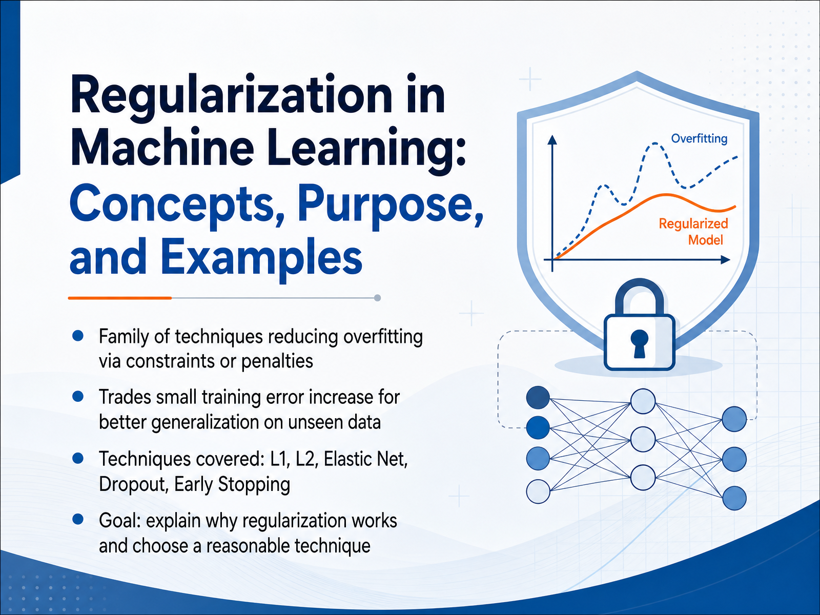
1. 01Regularization in Machine Learning: Concepts, Purpose, and ExamplesWelcome to this lesson on regularization in machine learning. I am glad you are here. Today we are going to explore a family of techniques that helps models perform better on new data, not just the data they were trained on. The core idea is simple. We gently constrain the model, or add a small penalty, so it does not fit the training examples too closely. In return, the model becomes better at generalizing to unseen examples. Yes, the training error may increase just a little, but that trade off is usually worth it. We will walk through five common techniques. L one, L two, Elastic Net, Dropout, and Early Stopping. The goal is not to memorize every formula. Instead, we want to understand why regularization works and how to choose a reasonable technique for your own model. Next, let us look at why regularization is needed in the first place.1 min
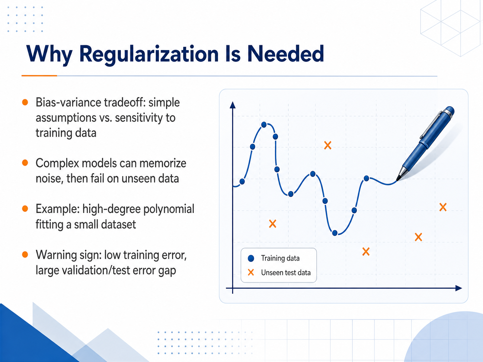
2. 02Why Regularization Is NeededLet's look now at why regularization is needed in the first place. In machine learning we often face a balance, sometimes called the bias-variance tradeoff. A very simple model may make strong assumptions and miss real patterns. A very complex model can become too sensitive to the training data. When that happens, the model starts to memorize noise instead of learning the underlying signal. Think of fitting a very high-degree polynomial to just a few data points. The curve may pass through every training point perfectly, but it can bend wildly in between and perform poorly on new examples. A clear warning sign is when training error is very low, but the validation or test error is much higher. That large gap usually tells us the model has overfit. Regularization helps close that gap by encouraging the model to stay simpler, which usually leads to better performance on unseen data. Next, we will explore the core idea behind this, which is adding a penalty term to the learning objective.1 min
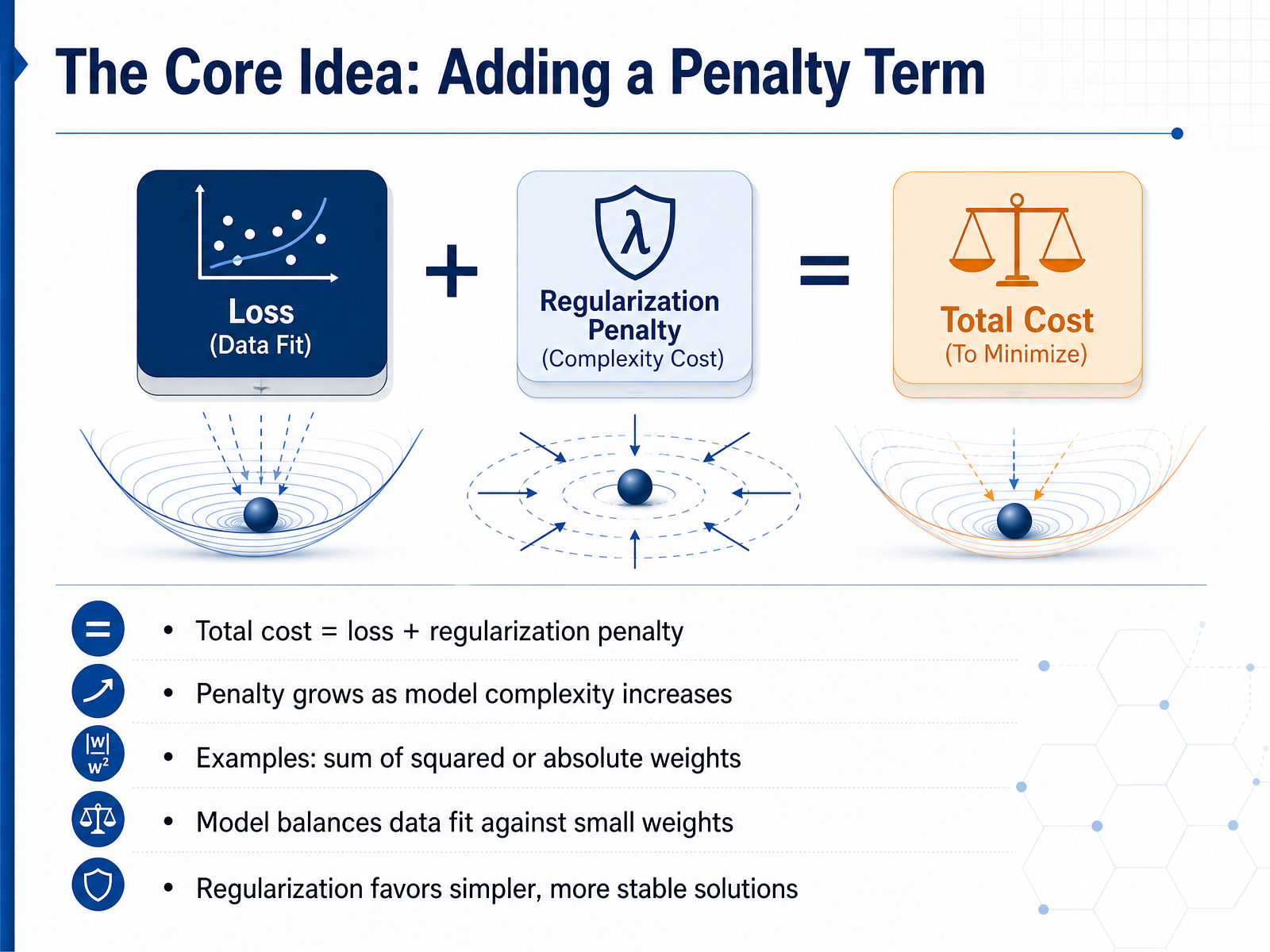
3. 03The Core Idea: Adding a Penalty TermNow let's look at the core idea behind regularization. We modify the training objective by adding a penalty term to the usual loss function. This means the total cost equals the original loss, plus a regularization penalty. The penalty grows as the model becomes more complex. For example, the penalty might be the sum of squared weights, or the sum of absolute weight values. Because the penalty grows with larger weights, the model is encouraged to keep weights small while still fitting the data well. In other words, the model balances fitting the training data against keeping the weights from becoming too large. This favors simpler and more stable solutions, which tend to generalize better to new data. Next, we'll explore the regularization parameter and why choosing it well matters.1 min
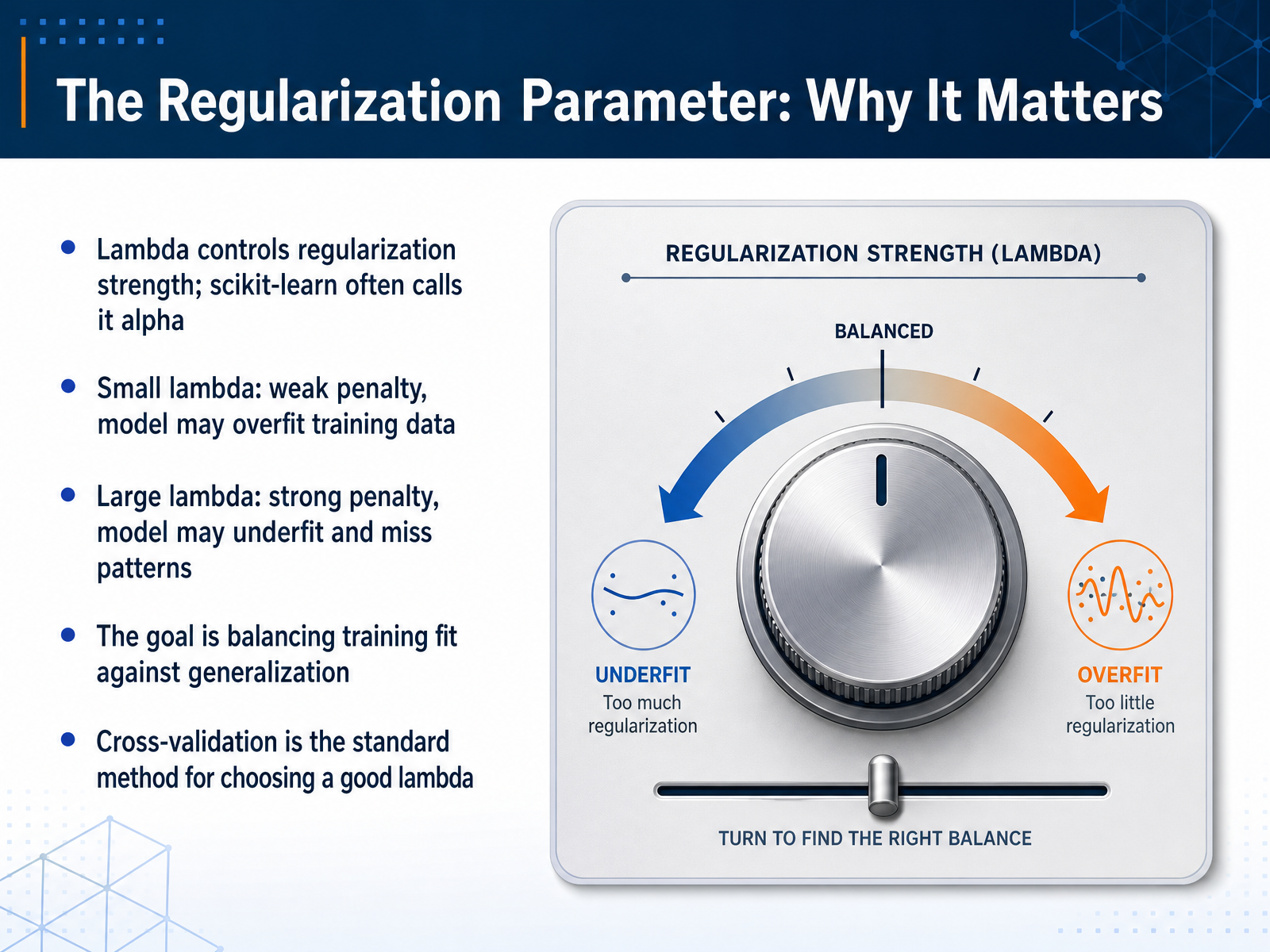
4. 04The Regularization Parameter: Why It MattersNow that we know a penalty term can help control complexity, let’s talk about the dial that controls its strength: the regularization parameter. In math we often call it lambda, and in scikit-learn you will often see it named alpha. Think of lambda as a volume knob. When lambda is small, the penalty is weak, so the model can fit the training data very closely. That may sound good, but it can capture noise and overfit. When lambda is large, the penalty is strong. The model becomes simpler, but if we push too far, it starts to underfit and misses real patterns in the data. So the real task is not making lambda as small or as large as possible. The goal is balance. We want a model that fits the training data well, but still generalizes to new examples. In practice, the standard way to find this balance is cross-validation. We try several values of lambda, evaluate the model on held-out folds, and choose the one that gives the most stable performance. With that foundation in place, we can look at two common ways to apply this penalty. Next, we turn to L1 regularization, also known as Lasso.1 min
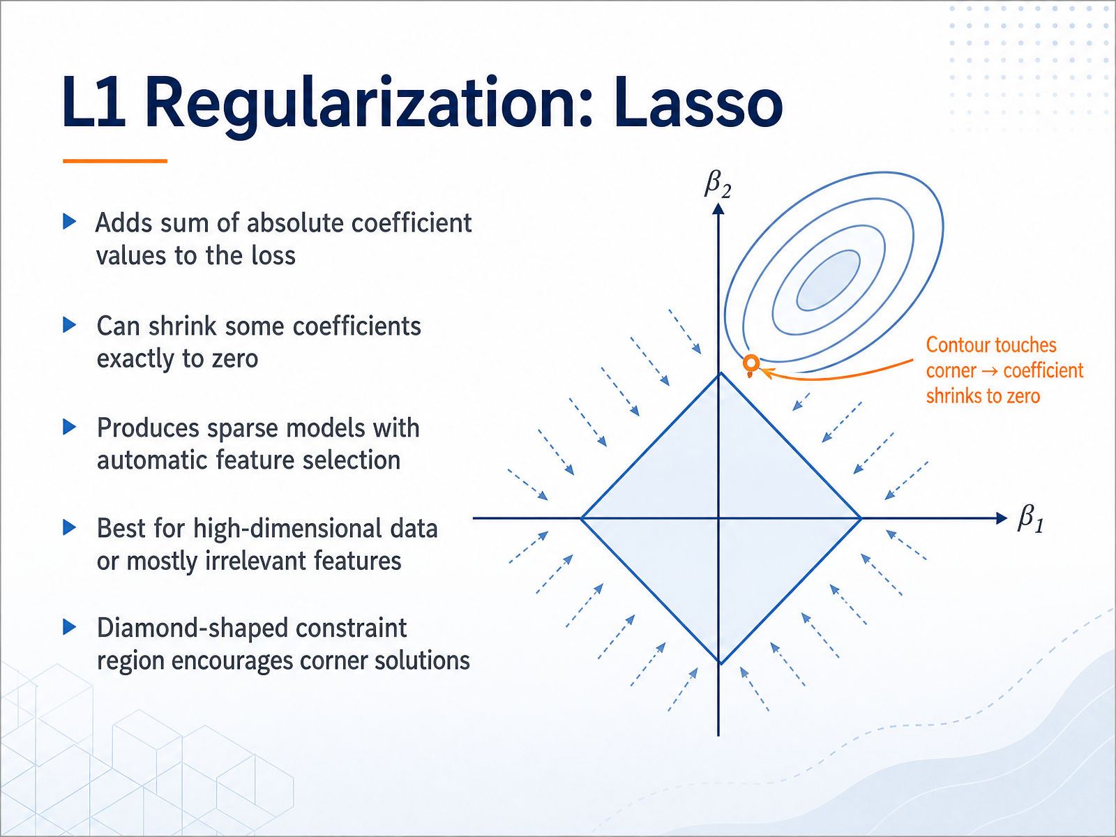
5. 05L1 Regularization: LassoNext, let's look at a specific form of regularization called L1 regularization, often known as Lasso. The idea is simple. We take the sum of the absolute values of all the model coefficients and add that sum to the loss function. Because we are adding a penalty based on coefficient size, the model is encouraged to keep coefficients small. But Lasso does something even more useful. With L1 regularization, some coefficients can be pushed all the way down to exactly zero. When a coefficient becomes zero, the corresponding feature no longer influences the prediction. This means Lasso can automatically perform feature selection for us. It is especially helpful when we have high dimensional data, such as hundreds or thousands of input variables, where many features may be irrelevant. Instead of manually deciding which features to keep, Lasso can remove them by setting their coefficients to zero. One helpful way to picture this is through the shape of the constraint region. For Lasso, the constraint region is diamond shaped, and that shape tends to encourage corner solutions, which is exactly where some coefficients hit zero. So the main takeaway is that L1 regularization produces sparse models and can automatically select useful features. Up next, we'll explore L2 regularization, also known as Ridge, which behaves a little differently.1 min
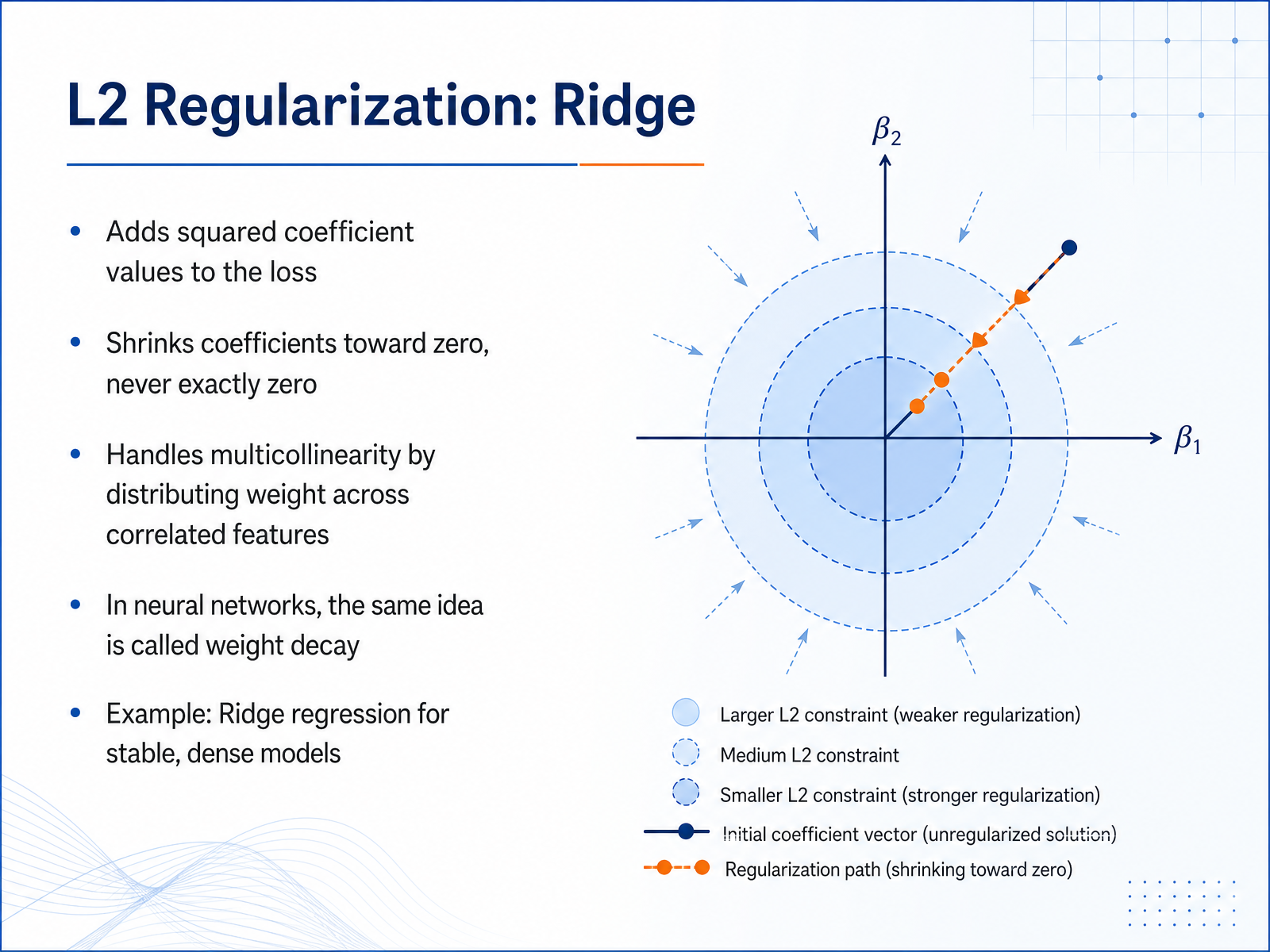
6. 06L2 Regularization: RidgeNext, we look at L2 regularization, often called Ridge regression. With L2, we add the squared values of the coefficients to the loss function. Think of it like a gentle pull toward zero. Because the penalty grows with the square of each weight, large weights become expensive, so the model shrinks them down. But here is the key difference: L2 rarely drives a coefficient all the way to zero. It shrinks them toward zero, but never exactly to zero. This is useful when features are correlated. Instead of picking one feature and ignoring the other, Ridge spreads the weight across all the correlated features, which makes the model more stable. In neural networks, the same idea is called weight decay, because the weights gradually decay toward smaller values during training. So when you want a stable, dense model that keeps all features but reduces their influence, Ridge regression is a great choice. Next, we will compare L1 and L2 side by side.2 min
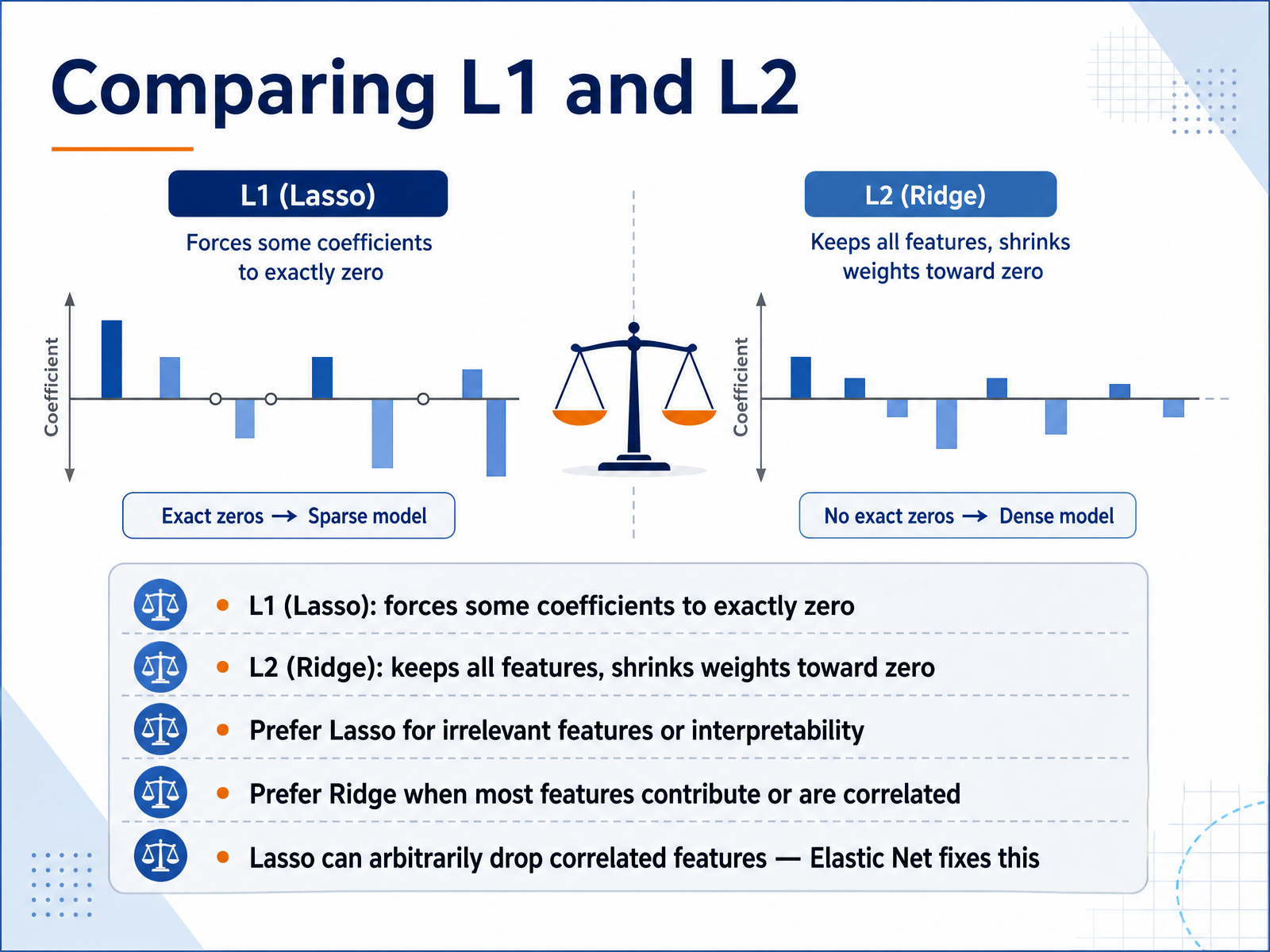
7. 07Comparing L1 and L2Now that we understand how regularization works, let's compare the two most common techniques: L1 and L2. Here is the main difference. L1 regularization, also called Lasso, can force some coefficients all the way to exactly zero. It acts like a feature selector, completely removing variables from the model. L2 regularization, or Ridge, works differently. It shrinks all the weights toward zero, but it typically keeps every feature in the model, just with a reduced influence. So how do we choose between them? If you suspect many features are irrelevant, or if you need a simple, interpretable model, Lasso is often the better choice because it can drop those features entirely. On the other hand, if you believe most features contribute at least a little, or if your features are highly correlated with each other, Ridge tends to be more stable. One caveat with Lasso is that when features are correlated, it can arbitrarily select one feature and drop the others, which may feel like losing valuable information. To address this specific issue, researchers combined both methods into something called Elastic Net. We will explore that combination next.1 min
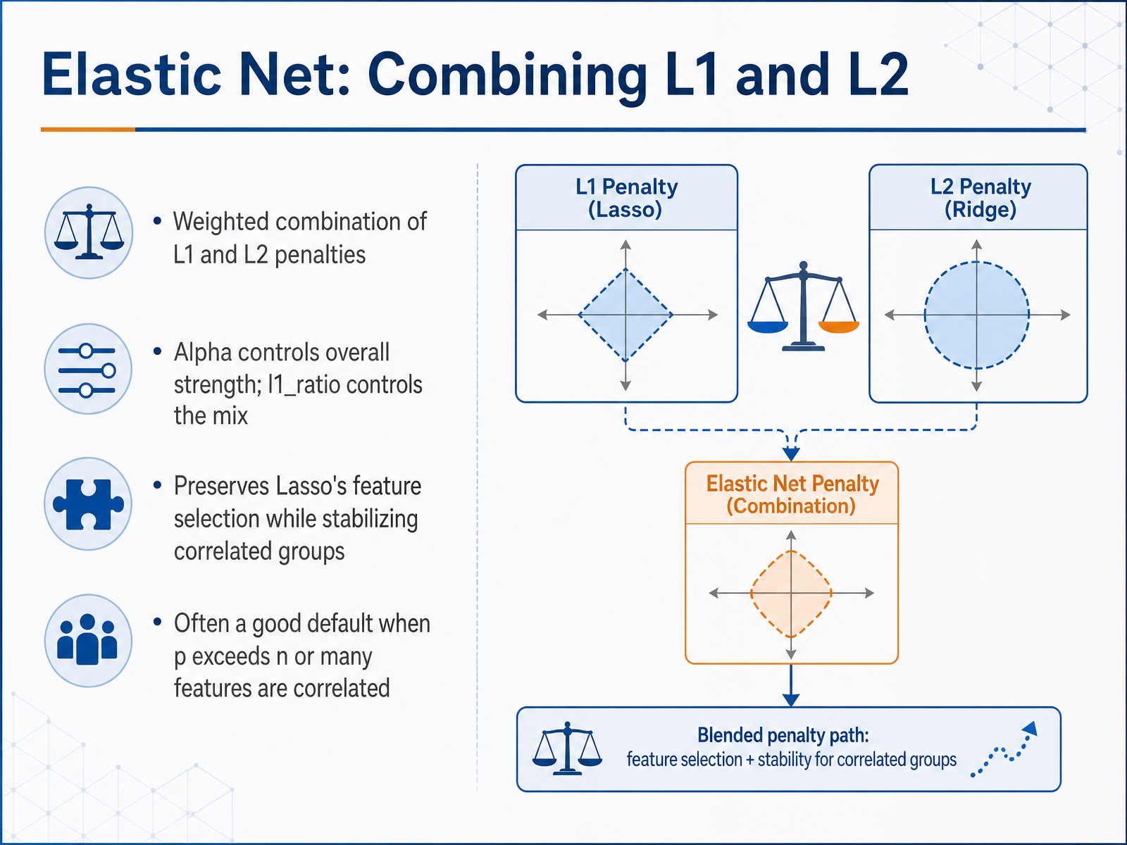
8. 08Elastic Net: Combining L1 and L2Now let's bring the two penalty approaches together. Elastic Net combines the L1 penalty from Lasso and the L2 penalty from Ridge into one weighted sum. Instead of choosing between feature selection and coefficient stability, we get a blend of both. Two parameters control this blend. Alpha sets the overall strength of regularization, so a larger alpha pulls the coefficients toward zero more strongly. The l1_ratio decides the mix. A higher l1_ratio behaves more like Lasso, encouraging sparse solutions. A lower l1_ratio behaves more like Ridge, smoothing coefficients especially among correlated features. This is useful when we have more predictors than observations, or when many features move together. Lasso alone may pick one feature from a correlated group almost at random, while Elastic Net can keep a small stable set instead. Because it balances sparsity and stability, Elastic Net is often a good default choice in these high-dimensional settings. Next, we'll look at how regularization extends beyond linear models.2 min
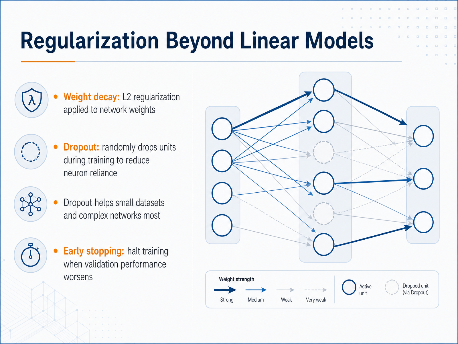
9. 09Regularization Beyond Linear ModelsRegularization ideas also extend beyond linear models. When we train neural networks, we often use a method called weight decay. This is essentially L2 regularization applied to the network's weights. Because the penalty grows with large weights, the network is encouraged to keep its parameters small and more balanced. Another powerful technique is dropout. During training, dropout randomly ignores a fraction of the neurons on each pass. This forces the network not to depend too heavily on any single neuron, so it learns more robust patterns. Dropout is especially helpful for small datasets and complex networks, where overfitting tends to be a bigger risk. We also have early stopping, which is simpler than it sounds. While training, we keep an eye on the validation performance. If it starts getting worse, we stop training, even if the training loss is still improving. This prevents the model from memorizing noise in the later training stages. So regularization in modern models often combines these ideas, controlling complexity from several angles at once. Next, we will look at a practical strategy for tuning and scaling these methods effectively.1 min
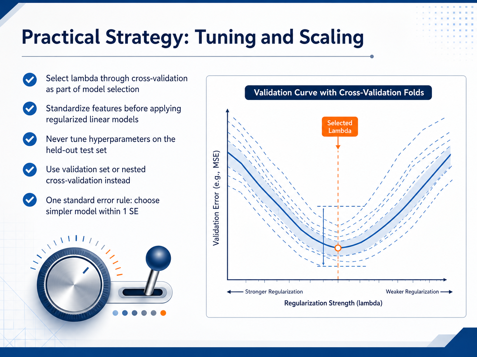
10. 10Practical Strategy: Tuning and ScalingNow let's focus on the practical side: how we actually choose and apply these techniques. First, the penalty strength, lambda, should be selected through cross-validation as part of model selection. Think of it as trying different levels of pressure on the model, and letting the data tell us which level generalizes best. Second, before we apply regularized linear models, we need to standardize the features. If one feature is measured in thousands and another in decimals, the penalty will hit them very differently, so scaling puts everyone on a fair playing field. Third, and this is crucial, we never tune hyperparameters on the held-out test set. The test set is our final report card, and if we peek at it while tuning, we lose that honest evaluation. Instead, use a dedicated validation set or nested cross-validation for tuning. Finally, there's a helpful shortcut called the one standard error rule. It says: if a simpler model performs within one standard error of the best model, prefer the simpler one. That keeps us from chasing tiny improvements that may just be noise. Up next, we'll look at common pitfalls and how to avoid them.2 min
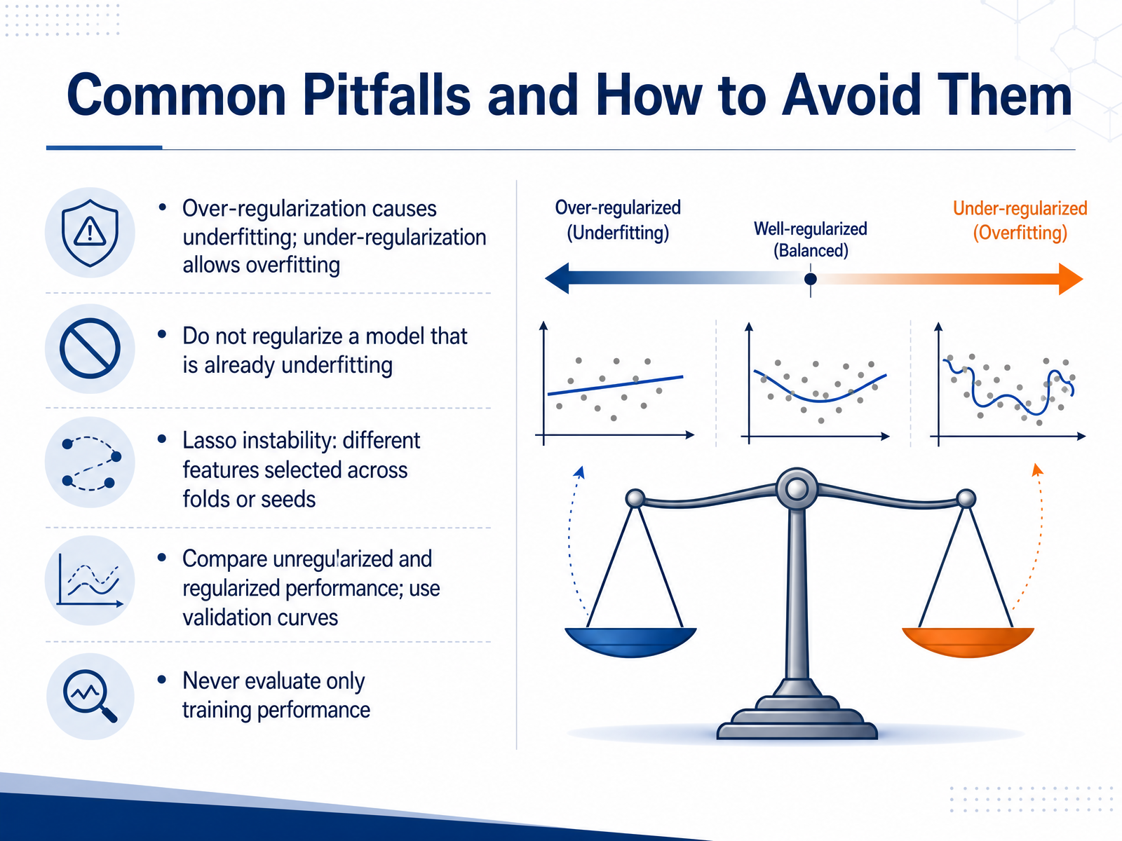
11. 11Common Pitfalls and How to Avoid ThemLet's look at some common pitfalls with regularization, and how to avoid them. First, balance matters. If we push the penalty too hard, the model becomes too simple and misses important patterns. That's underfitting. If the penalty is too weak, the model stays too flexible and chases noise. That's overfitting. So we need to find the middle ground. Also, avoid applying strong regularization to a model that is already underfitting. That just makes the problem worse. Another issue is instability in Lasso. Because Lasso can shrink some coefficients all the way to zero, small changes in the data or random splits can lead to different features being selected across different cross-validation folds or random seeds. That can make interpretation tricky. So how do we catch these issues? Always compare regularized performance against an unregularized baseline. Use validation curves to see how performance changes as the penalty strength increases. And never judge a model by training performance alone. Always check validation or test results. In short, regularization requires tuning, not just turning it on. Next, we'll walk through a worked example with linear regression to see these ideas in practice.2 min
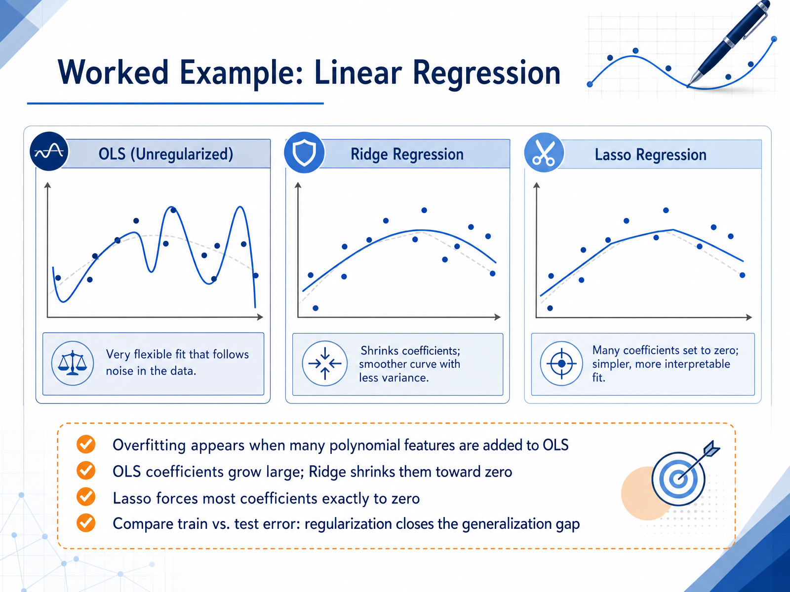
12. 12Worked Example: Linear RegressionNow let's see regularization in action with a classic linear regression problem. What happens if we add many polynomial features to ordinary least squares? The model becomes too flexible, and it starts fitting the noise in the training data. We can spot this because the coefficients grow very large, almost as if the model is straining to bend itself around each data point. Ridge regression fixes this by adding a penalty on the size of the coefficients, which shrinks them toward zero and smooths out the curve. Lasso goes one step further. It also shrinks coefficients, but because of how its penalty works, it often pushes most of them exactly to zero. This makes Lasso a great tool for automatic feature selection. The crucial test is performance. When we compare training error against test error on a held out set, the overfit model has low training error but high test error. After applying regularization, the gap between the two errors closes. That gap is what we call the generalization gap, and narrowing it is a major goal in machine learning. Next, we will apply these same ideas to a more complex model, a neural network.1 min
13. 13Worked Example: Regularizing a Neural NetworkNow let's see regularization in action on a neural network. Imagine we have a small, noisy dataset, and our network learns it too aggressively. It starts fitting every random bump and outlier, so training accuracy looks great, but validation accuracy drops. That is overfitting. One practical remedy is dropout. During training, dropout randomly disables some units on each pass. Because the network cannot rely on any single neuron, it is forced to spread out what it learns, almost like studying with a changing study group instead of one fixed set of notes. If we then plot training and validation curves, the gap between them usually shrinks. That smaller gap is our sign that the model is generalizing better. Next, early stopping gives us another guardrail. We watch validation loss while training, and as soon as it starts to worsen consistently, we halt. You can think of it as stepping away from the oven once the cake is perfectly baked, instead of leaving it until the edges burn. And for a fuller picture, dropout changes the network structure during training, while weight decay quietly shrinks the weights themselves. Together, they push the model toward simpler, more stable patterns. With this concrete example in mind, let's move to the final slide and bring everything together with a summary and next steps.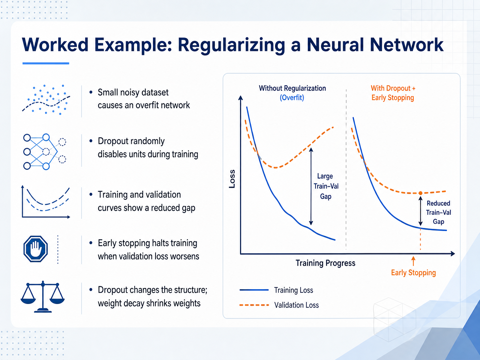2 min
14. 14Summary and Next StepsLet’s bring everything together. Regularization is really about one trade off. We accept a small increase in bias, meaning the model is a little less flexible, and in return we get a much larger reduction in variance, so the model is far more stable on new data. The main techniques we covered are Lasso and Ridge, which add a penalty to the size of the coefficients. Elastic Net combines both ideas. Dropout works differently by randomly turning off neurons during training, and Early Stopping simply pauses training before the model begins to memorize noise. How do you choose? If you suspect only a few features matter, Lasso can help by shrinking some coefficients to zero. If features are correlated or you have a smaller dataset, Ridge or Elastic Net often work better. The next step is to tune the penalty strength using cross validation, and then compare training error against test error to make sure the gap is closing. The best way to make this real is to practice. The scikit-learn and Keras tutorials are beginner friendly and will walk you through each technique. Thank you for staying with me through this topic. You now have a practical toolkit for building models that generalize. Keep experimenting, and you’ll build intuition faster than you expect.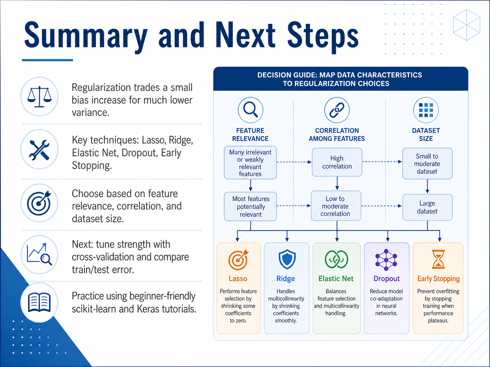2 min