X Bar in Statistics: Concepts and Examples

Learn the statistical concept, purpose, and practical applications of the X-bar chart for monitoring sample means in quality control.

A digital instructor presents all 14 pages. Hold “Ask” at any point and ask out loud — the answer comes from this course. No sign-up needed.

28 minFree to watchDownloads

What you’ll learn

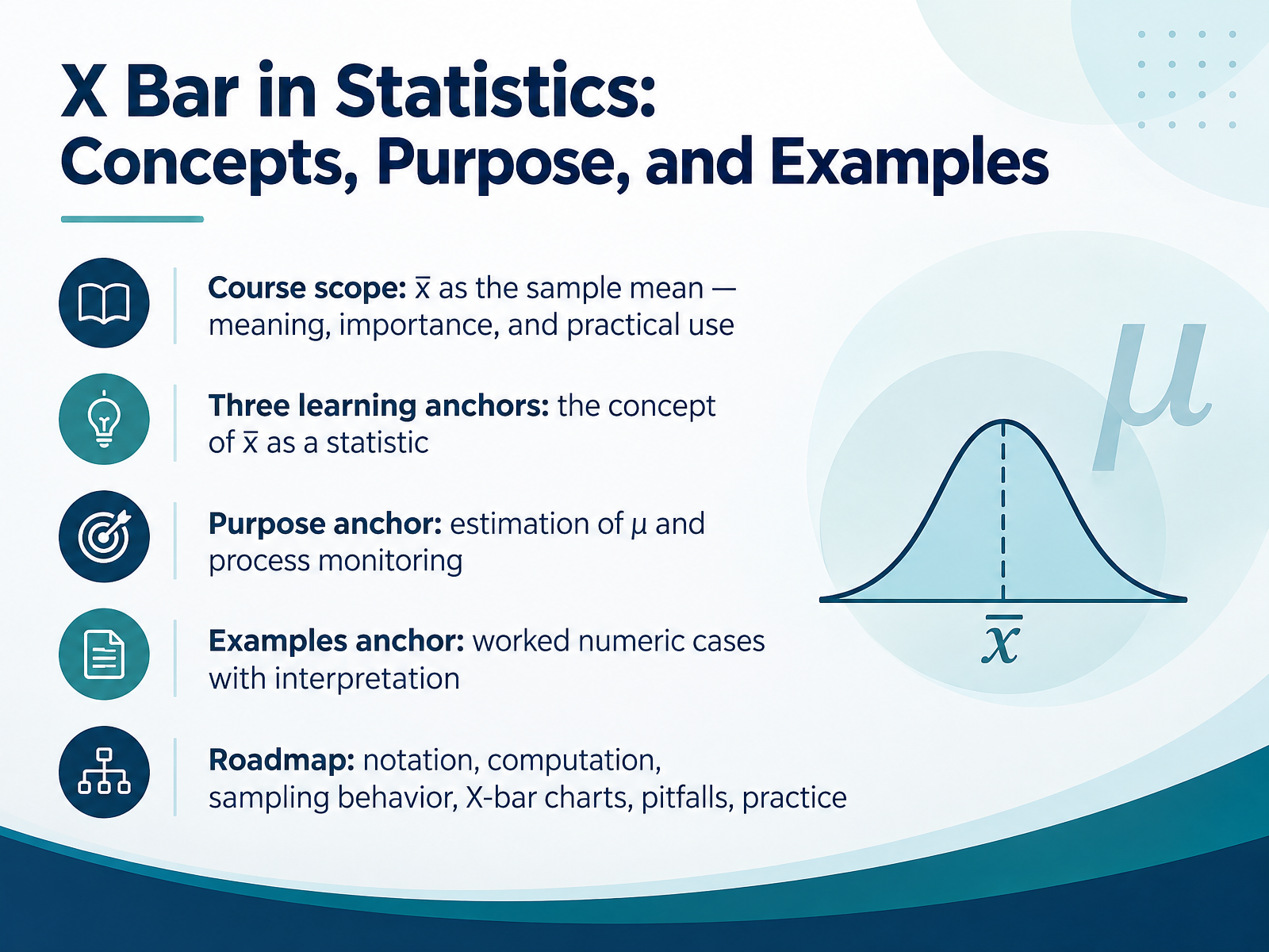
01X Bar in Statistics: Concepts, Purpose, and ExamplesWelcome. I'm glad you're here. In this course, we'll build a clear, practical understanding of x bar, the sample mean. Our goal is simple: by the end, you'll know what x bar measures, why it matters, and how to use it with confidence in quality or research work. Along the way, we'll rely on three anchors. First, the concept: x bar is a statistic, a number computed from a sample. Second, the purpose: estimating the population mean, mu, and monitoring processes over time. Third, examples: worked numeric cases, with interpretation, so the ideas stick. One quick note before we begin. A common misconception is that any single sample mean should equal the population mean. In fact, x bar varies from sample to sample, and larger samples usually produce less variability. We'll revisit that carefully. Here's your takeaway for this opening. Whenever you see x bar, ask three questions: What sample produced it, what is it estimating, and how much could it vary? Keep those questions in mind, and the rest of the course becomes much easier to follow. Next, we'll look at where x bar comes from, in From Population to Sample: Where X Bar Fits.doi.org jse.amstat.org files.eric.ed.gov+22 min
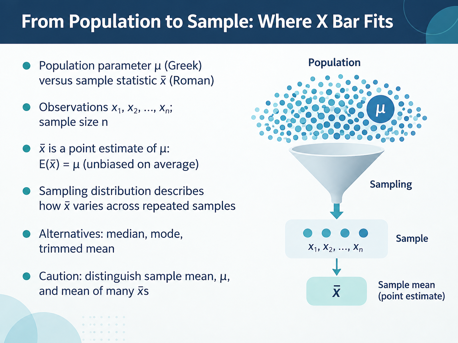
02From Population to Sample: Where X Bar FitsNow let's connect the dots from population to sample. A population parameter, written with the Greek letter mu, is a fixed but usually unknown value, like the true average fill volume of every bottle on a production line. The sample statistic, written as x bar, is what you calculate from the observations x one, x two, up to x n, where n is your sample size. X bar is a point estimate of mu, and on average it equals mu, which is what unbiased means. But any single sample mean will vary, and the sampling distribution describes that variation across repeated samples. Other options exist, such as the median, mode, or trimmed mean. Here is the caution. Keep the sample mean, the population mean mu, and the mean of many x bars distinct, because mixing them up is a very common misconception. Your takeaway: state clearly which mean you are working with before you interpret any result. Next, we will compute x bar using the formula and weighted variants.doi.org jse.amstat.org files.eric.ed.gov+22 min
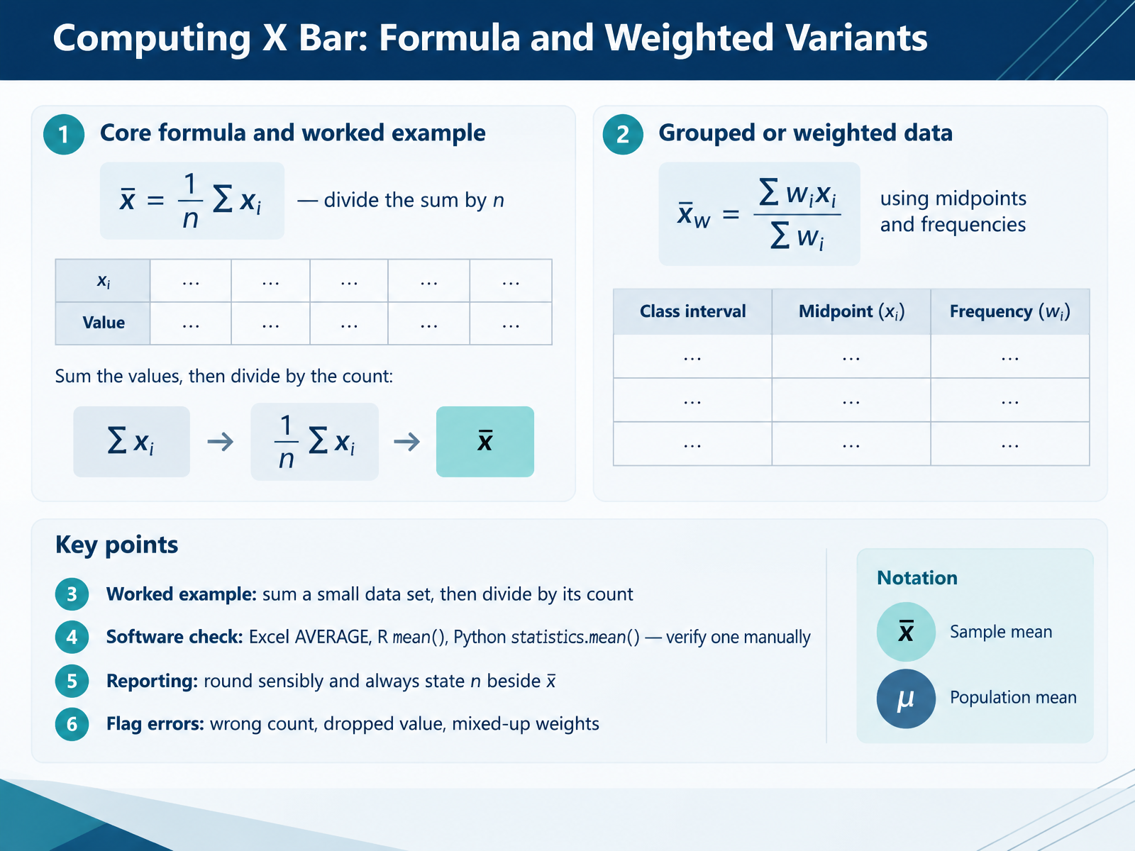
03Computing X Bar: Formula and Weighted VariantsNow let's look at how X bar is actually computed. The core formula is simple: x bar equals the sum of all values divided by n, the number of values. For example, with the numbers four, six, eight, and ten, the sum is twenty eight, and dividing by four gives an X bar of seven. When data come grouped, use a weighted version: multiply each midpoint by its frequency, sum those products, then divide by the total frequency. Software makes this easy, but verify one result by hand, because common errors include using the wrong count, dropping a value, or mixing up weights. So always report X bar with its n, rounded sensibly. Next, we'll explore why X bar matters and how to interpret it.doi.org jse.amstat.org files.eric.ed.gov+21 min
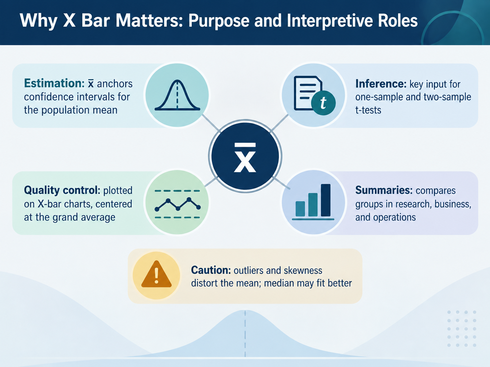
04Why X Bar Matters: Purpose and Interpretive RolesNow let's look at why x-bar matters and how you can interpret it. X-bar serves five practical roles. First, estimation. x-bar anchors confidence intervals for the population mean, giving you a plausible range for that unknown value. Second, inference. x-bar is a key input for one-sample and two-sample t-tests, which compare means across groups. Third, quality control. On an X-bar chart, subgroup means are plotted and centered at the grand average, often written as x double bar. Here is a caution: examine the range chart first. If variability is out of control, the X-bar limits are unreliable. Fourth, summaries. x-bar compares groups in research, business, and operations, such as average wait times by shift. Finally, caution. Outliers and skewness distort the mean, so the median may fit better. A common misconception is that x-bar should equal the population mean in every sample, but it varies from sample to sample. Also, control limits are not specification limits. Your takeaway: before trusting x-bar, check the data shape and process stability, and report the median alongside it when the data are skewed. Next, we examine how x-bar behaves across repeated samples in Sampling Behavior: Standard Error and the Central Limit Theorem.itl.nist.gov web.mit.edu doi.org+22 min
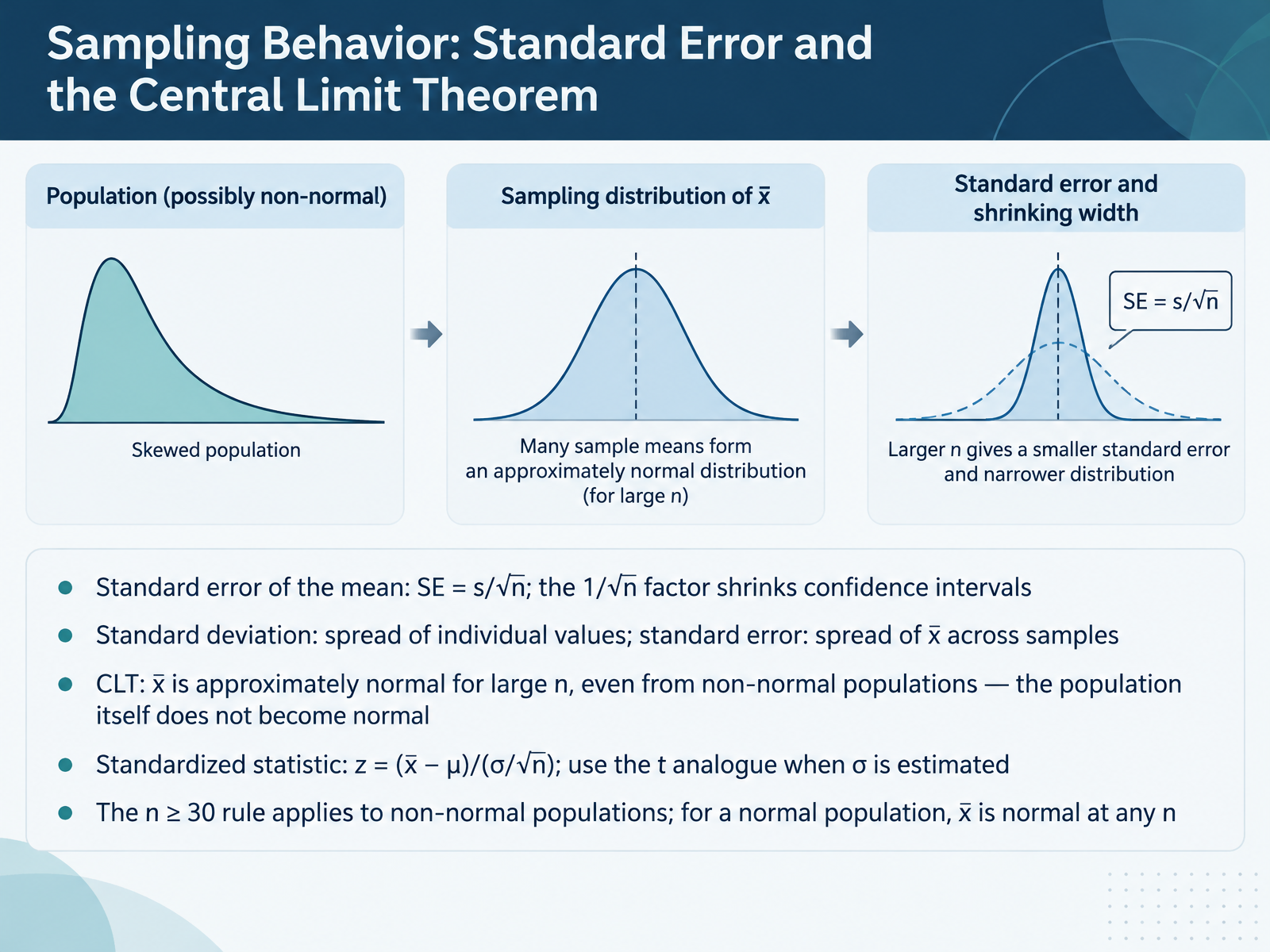
05Sampling Behavior: Standard Error and the Central Limit TheoremNow let's look at how x-bar behaves from sample to sample. First, standard error of the mean. It equals s divided by the square root of n. That one over root n factor is why larger samples give narrower confidence intervals. For example, quadrupling your sample size halves the standard error. Next, keep two spreads separate. Standard deviation describes how individual values vary. Standard error describes how x-bar varies across repeated samples. Then the central limit theorem. For large n, x-bar is approximately normal, even when the population is not. But the population itself does not become normal. To standardize, z equals x-bar minus mu divided by sigma over root n, and you use the t analogue when sigma is estimated. One assumption to check: n greater than or equal to thirty is a guideline for non-normal populations. If the population is already normal, x-bar is normal at any sample size. Your takeaway: report standard error, which is sample size dependent, not standard deviation, when describing the precision of a mean. This sets up the common misconceptions we'll address next, in Misconceptions About Sampling Behavior to Address Early.doi.org jse.amstat.org files.eric.ed.gov+22 min
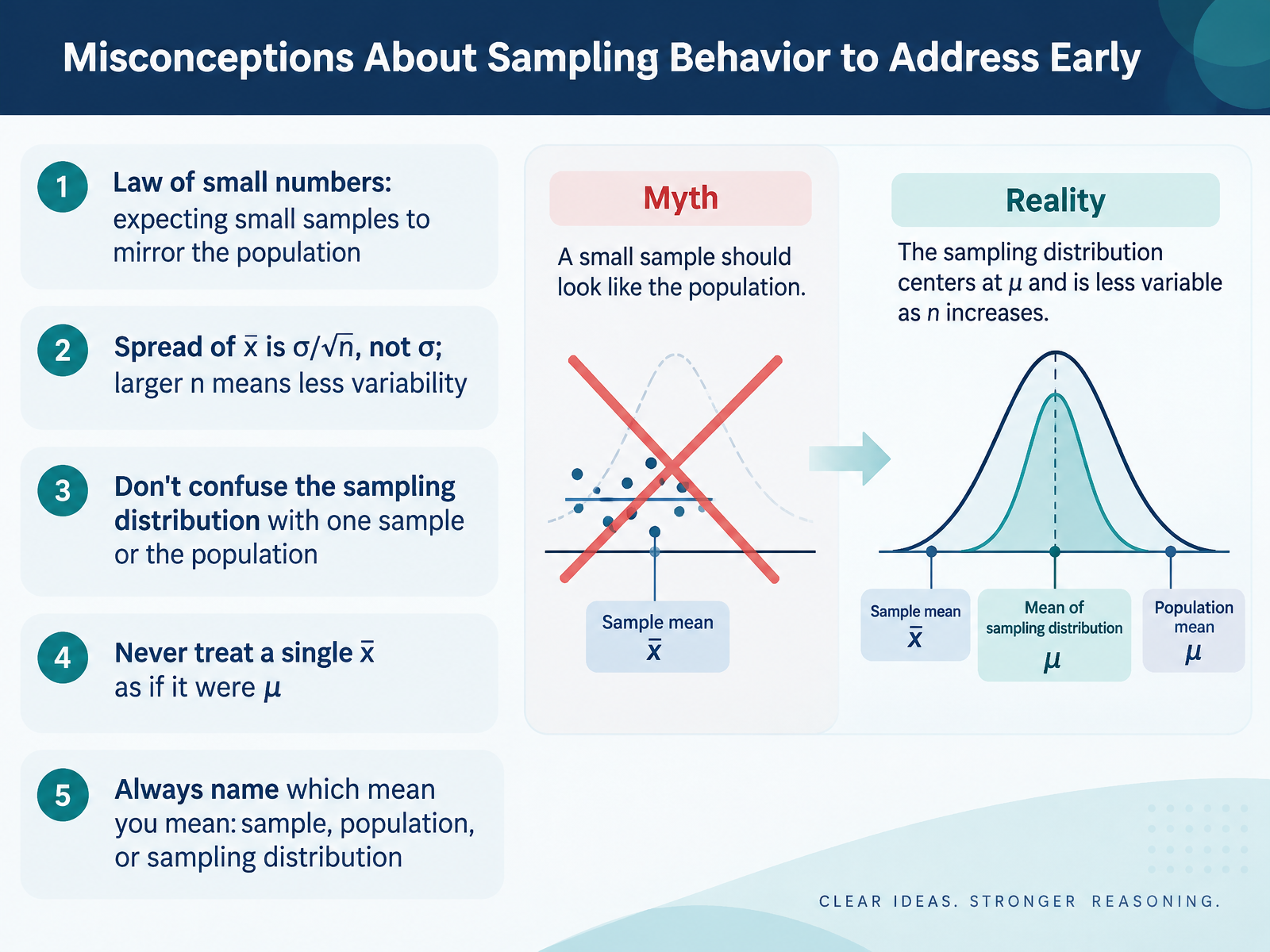
06Misconceptions About Sampling Behavior to Address EarlyBefore we go further, let's clear up several misconceptions about sampling behavior that trip people up early. First is the law of small numbers: the false belief that a small sample should mirror the population. It won't. Flip a coin ten times and you may easily get seven heads; that doesn't mean the coin is unfair. Second, the spread of x bar is sigma divided by the square root of n, not sigma itself. As n grows, sample means cluster more tightly around mu. Third, don't confuse the sampling distribution with one sample or with the population. The sampling distribution is the pattern of many sample means, not a single result. Fourth, never treat a single x bar as if it were mu. One sample mean is an estimate, and it varies from sample to sample. Finally, always name which mean you mean: the sample mean, the population mean, or the mean of the sampling distribution. A practical takeaway: before interpreting any mean, label it, and remember that larger samples reduce variability, not bias. Next, we'll apply x bar in quality control by examining chart structure and control limits.doi.org jse.amstat.org files.eric.ed.gov+22 min
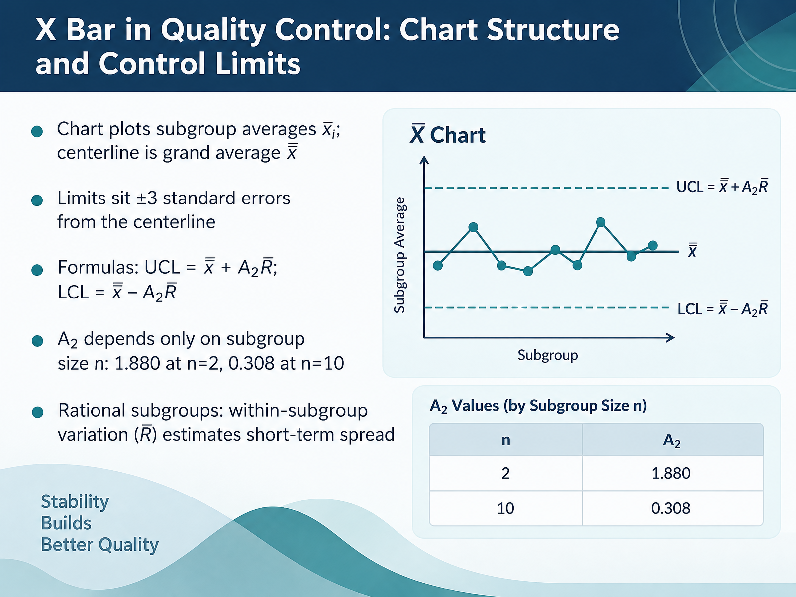
07X Bar in Quality Control: Chart Structure and Control LimitsNow let's look at the structure of an X-bar chart and how its control limits are built. Each point on the chart is a subgroup average, x-bar sub i, plotted over time. The centerline is the grand average, x-bar bar, the mean of all those subgroup averages. The limits sit three standard errors above and below the centerline, which gives an upper limit of x-bar bar plus A two times R bar, and a lower limit of x-bar bar minus A two times R bar. Here R bar is the average range, and A two is a constant that depends only on subgroup size. At n equals two, A two is one point eight eight zero. At n equals ten, it drops to zero point three zero eight. One common misconception is that these are specification limits. They are not. They describe the process's own variation. That variation comes from rational subgroups: groups chosen so that conditions inside each group are alike, so the within-subgroup spread, R bar, estimates short-term variation. So before you interpret the X-bar chart, confirm your subgroups are rational and check the range chart first. Next, we will look at paired charts, X-bar with R or s, and how to read their signals.itl.nist.gov web.mit.edu doi.org+22 min
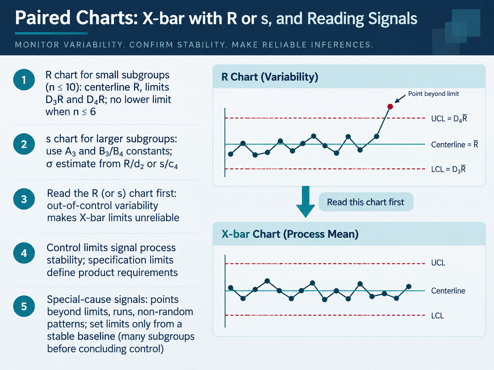
08Paired Charts: X-bar with R or s, and Reading SignalsNow let's look at reading the charts together. An X bar chart almost always travels with a companion chart for variability: the R chart when your subgroups are small, roughly ten or fewer, and the s chart for larger subgroups. The R chart uses the average range as its centerline, with limits at D three times R bar and D four times R bar. When n is six or less, the lower limit is effectively zero, so there is no lower limit to plot. The s chart uses A three and B three and B four constants. You estimate sigma from R bar divided by d two, or from s divided by c four. Here is the habit that matters most: read the variability chart first. If the R or s chart shows an out-of-control condition, the X bar limits built from that data are unreliable. Also keep two ideas separate. Control limits tell you whether the process is stable. Specification limits define what the product requires. And remember, special-cause signals include points beyond the limits, runs, and non-random patterns, and you should set limits only from a stable baseline with many subgroups. So before drawing any conclusion, check the variability chart, then the average. Next, we will work through a full example: computing and interpreting X bar.itl.nist.gov web.mit.edu doi.org+22 min
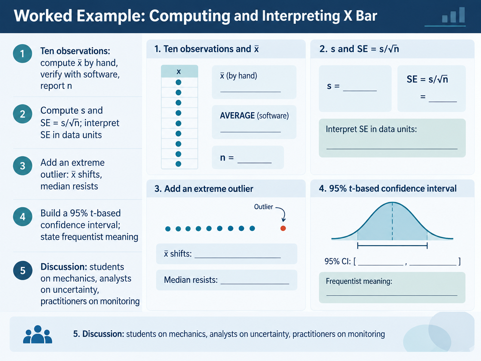
09Worked Example: Computing and Interpreting X BarNow let's put X bar to work with a hands-on example. Suppose you collect ten observations. Compute x bar by hand, then verify it in software, and always report n, the number of observations. Next, calculate the standard deviation, s, and the standard error, which is s divided by the square root of n. The standard error is in your data's units, so it describes how much sample means are expected to vary from sample to sample, not how much individual values vary. Now add one extreme outlier. Watch what happens. X bar shifts toward the outlier, while the median resists. This is why you inspect your data before trusting a mean. Finally, build a ninety-five percent t-based confidence interval and say what it means: if we repeated sampling many times, about ninety-five percent of intervals built this way would contain the true mean. For students, practice the mechanics. For analysts, focus on uncertainty. For practitioners, monitor what happens over time. Next, we build an X bar chart from subgroups.doi.org jse.amstat.org files.eric.ed.gov+22 min
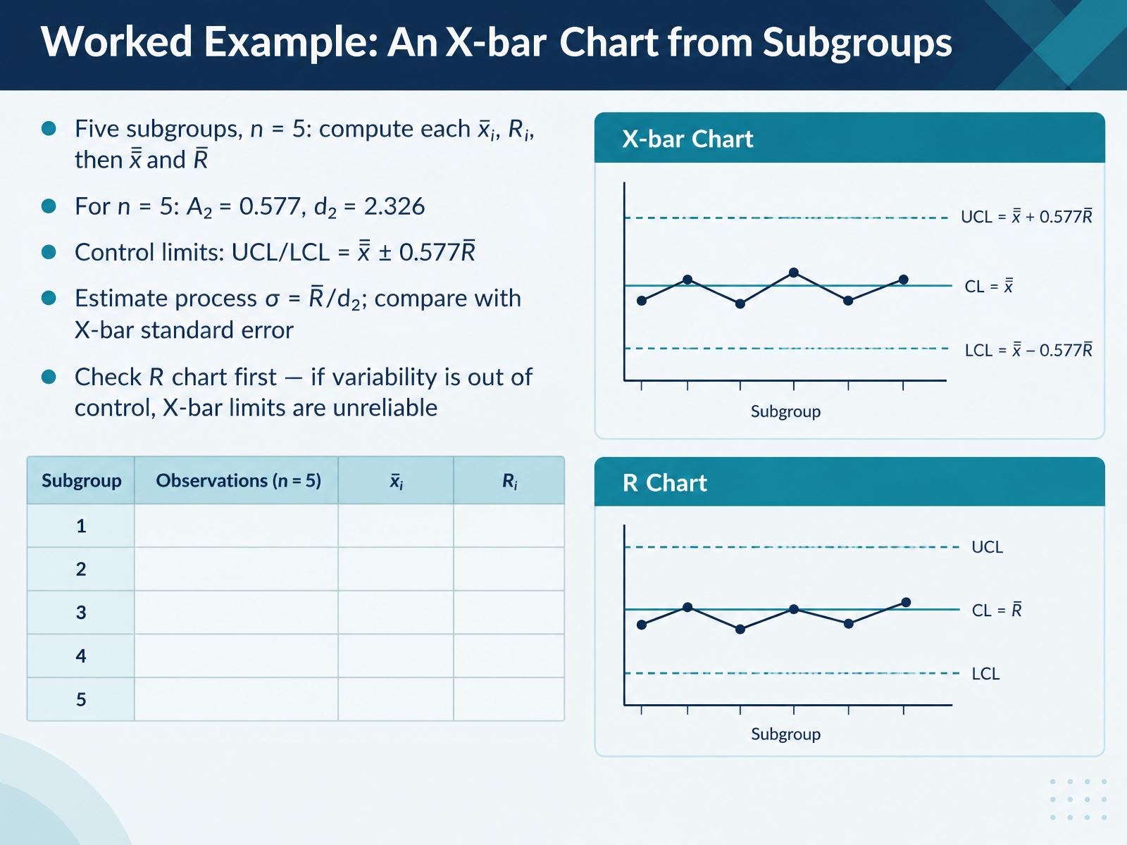
10Worked Example: An X-bar Chart from SubgroupsNow let's walk through a worked example, building an X-bar chart from subgroups. Suppose you collect five subgroups, each with five measurements, so n equals five. For each subgroup, compute the average, x-bar sub i, and the range, R sub i. Then average those five averages to get the grand average, x-bar bar, and average the ranges to get R bar. With n equals five, use two constants from the table: A two equals zero point five seven seven, and d two equals two point three two six. The control limits are x-bar bar plus or minus zero point five seven seven times R bar. You can also estimate the process standard deviation as R bar divided by d two. Compare that with the standard error of the X-bar chart, which is sigma divided by the square root of n. Here is the key practice point: check the R chart first. If variability is out of control, the X-bar limits are unreliable, so fix the variation before judging the average. Next, we will look at common pitfalls and best practices.itl.nist.gov web.mit.edu doi.org+21 min
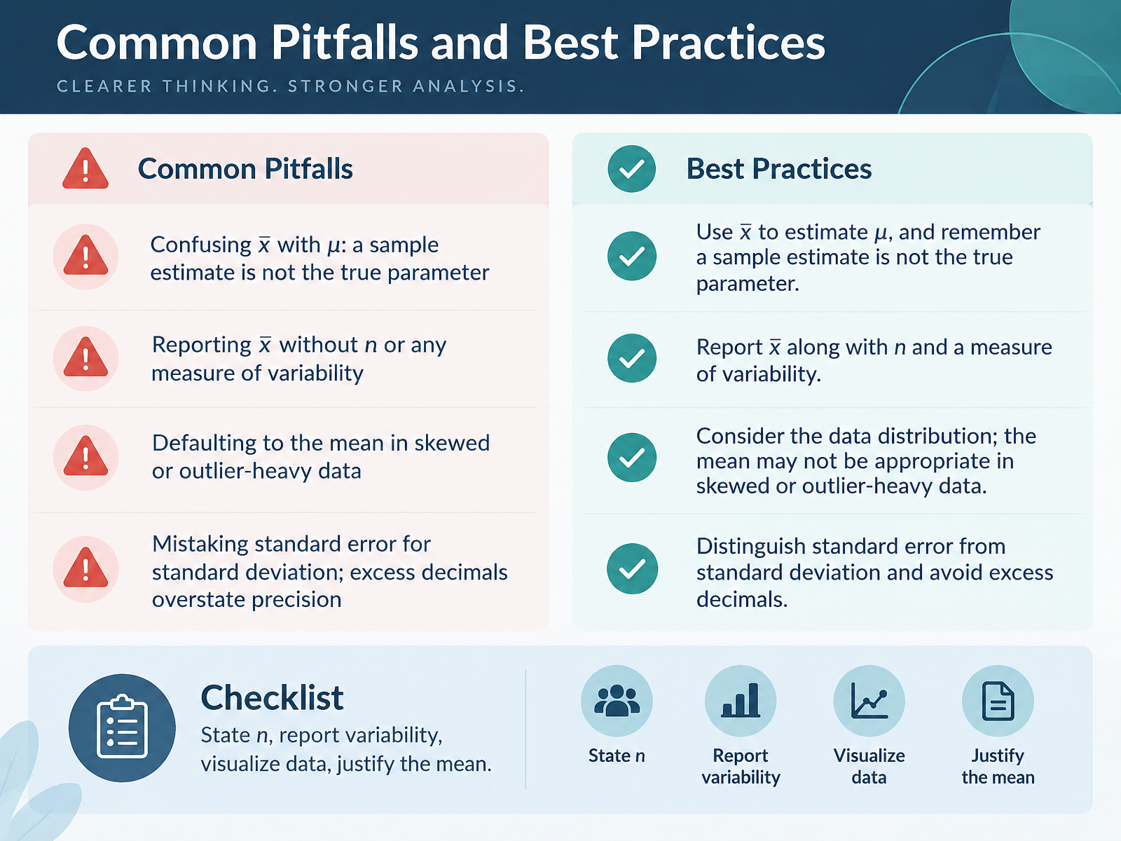
11Common Pitfalls and Best PracticesNow that you know how to compute x-bar, let's look at where interpretations commonly go wrong, and how to avoid them. First, don't confuse x-bar with mu. X-bar is a sample estimate; mu is the true, unknown population mean. A single sample gives you an estimate, not the parameter itself. Second, never report x-bar alone. Always state the sample size, n, and some measure of variability, because a mean without spread hides how reliable it is. Third, don't default to the mean when your data are skewed or contain outliers. In those cases, the median may describe the typical value far better. Fourth, don't mistake standard error for standard deviation. Standard error measures how much x-bar varies from sample to sample, while standard deviation describes variation among individual observations. And avoid excess decimals; reporting too many implies a precision you don't have. Here's a simple checklist: state n, report variability, visualize the data, and justify why the mean is appropriate. Carry that checklist into the next slide, Case Study: When the Mean Misleads.itl.nist.gov web.mit.edu doi.org+22 min
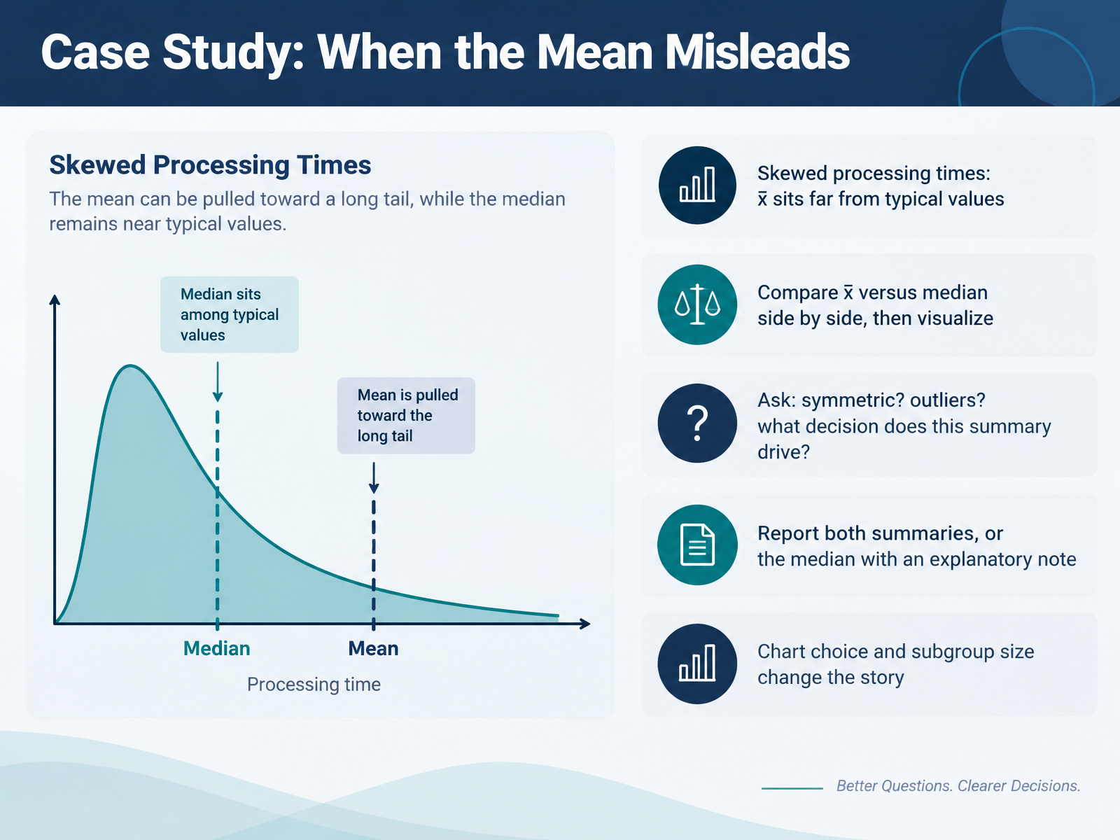
12Case Study: When the Mean MisleadsLet's look at a real case where the mean can mislead you. Suppose you are tracking processing times, and the distribution is skewed, with a few very slow jobs stretching the tail to the right. In that situation, x bar, the sample mean, can sit far from the typical value most jobs actually take, because it gets pulled toward those extreme observations. Here is a practical check. Compare x bar and the median side by side, then visualize both on the same histogram or dot plot. Ask yourself three questions. Is the data symmetric? Are there outliers? And what decision will this summary drive? For skewed data, report both summaries, or report the median with a short explanatory note. Keep in mind that your chart choice and subgroup size change the story, so never let one number speak alone. Now let's test your understanding with Practice and Assessment: Check Your Understanding.doi.org jse.amstat.org files.eric.ed.gov+21 min
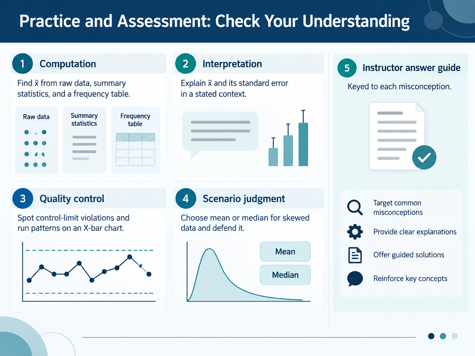
13Practice and Assessment: Check Your UnderstandingNow let's put everything into practice with a short self-check. First, computation. You should be able to find x-bar from raw data, from summary statistics, and from a frequency table. For example, with a frequency table, multiply each value by its frequency, add those products, then divide by the total count. Second, interpretation. Explain x-bar and its standard error in a stated context, remembering that standard error measures how much sample means vary, not how much individual values vary. Third, quality control. On an X-bar chart, spot points outside the control limits and nonrandom run patterns, and check the R chart first, because unstable variation makes the X-bar limits unreliable. Fourth, scenario judgment. Choose the mean or the median for skewed data and defend your choice. The instructor answer guide is keyed to each common misconception, such as assuming every sample mean must resemble the population. A useful takeaway is to write your reasoning, not just your answer, so feedback targets the right idea. Next, we'll consolidate with Key Takeaways and Next Steps.itl.nist.gov web.mit.edu doi.org+22 min
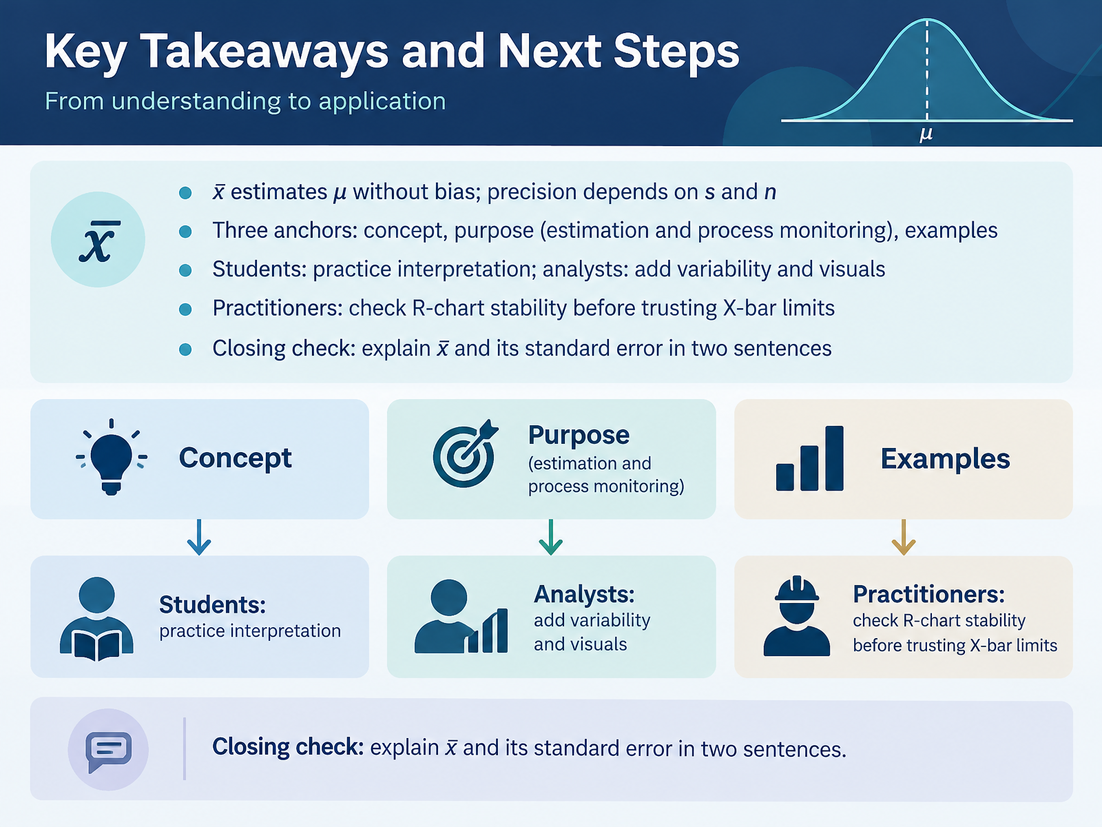
14Key Takeaways and Next StepsLet's bring everything together. X-bar estimates the population mean, mu, without bias, and its precision depends on the spread of the data and on sample size. When n grows, x-bar varies less from sample to sample. That is why the standard error shrinks as n increases. Remember the three anchors: the concept of x-bar, its purpose in estimation and process monitoring, and worked examples. If you are a student, practice reading x-bar values in context, not just calculating them. If you are an analyst, always report variability and visuals alongside the mean. And if you are a practitioner, check the R chart first. If the ranges are unstable, the X-bar limits are unreliable, because the limits use the average range. Your closing check: explain x-bar and its standard error in two sentences. For example, x-bar is the average of a sample and estimates the population mean. Its standard error measures how much x-bar varies between samples, and it gets smaller as sample size increases. Thank you for learning with me. Keep practicing, question your charts, and your interpretation skills will keep improving.itl.nist.gov web.mit.edu doi.org+22 min

Take the deck with you

Download this course as a file — free, no sign-up needed.

PDF handoutEvery slide page, ready to print or share.15 pages · 3.1 MBDownload
Narrated PowerPointThe deck that presents itself — every slide carries the digital human's narration video.15 pages · 14.6 MBDownload
PowerPoint slidesThe full deck as a .pptx — open it in PowerPoint, Keynote, or Google Slides.15 pages · 3.0 MBDownload

Free to use in your own training — please keep the PersonWise credit page at the end.

Have your own deck? Turn it into a course

Sources consulted

Web sources consulted while building this course.