Statistical Parameters: Concepts and Examples

This training explains statistical parameters, their purpose, and practical examples for learners seeking a clear foundation in statistical concepts.

My workspace30 minFree to watchDownloads

What you’ll learn

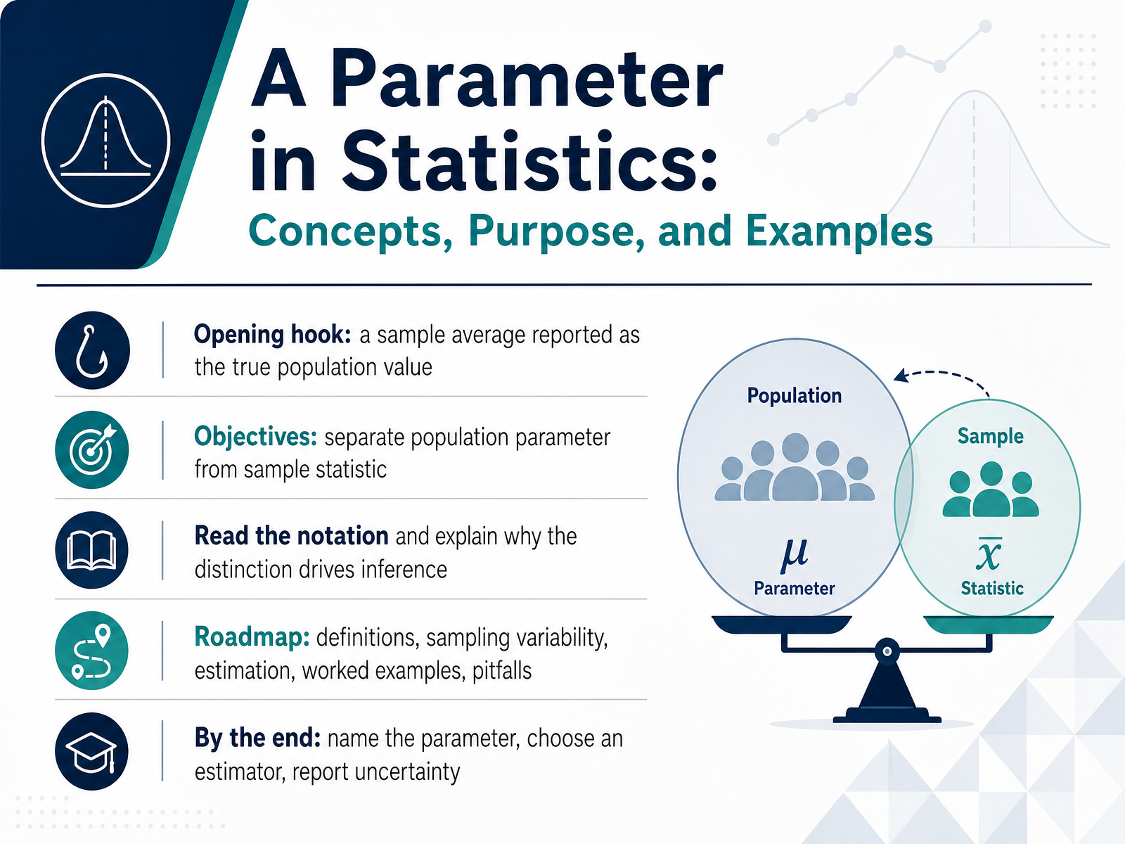
01A Parameter in Statistics: Concepts, Purpose, and ExamplesWelcome. I'm glad you're here. Today we're tackling one of the most important distinctions in all of statistics: the difference between a population parameter and a sample statistic. Here's the hook. Someone reports a sample average, like a mean rent of one thousand two hundred dollars, and then talks about it as if it were the true value for everyone. That small slip causes big problems. So our objectives are practical. You'll learn to separate a parameter, a number that describes an entire population, from a statistic, a number calculated from a sample. You'll read the standard notation, like mu for a population mean and x bar for a sample mean, and you'll see why this distinction drives statistical inference. Here's our roadmap. We'll cover definitions, sampling variability, estimation, worked examples, and common pitfalls. By the end, you'll be able to name the parameter, choose an appropriate estimator, and report uncertainty honestly. Let's begin with what a parameter is, and what a statistic is.exploration.stat.illinois.edu pressbooks.cuny.edu courses.lumenlearning.com+21 min
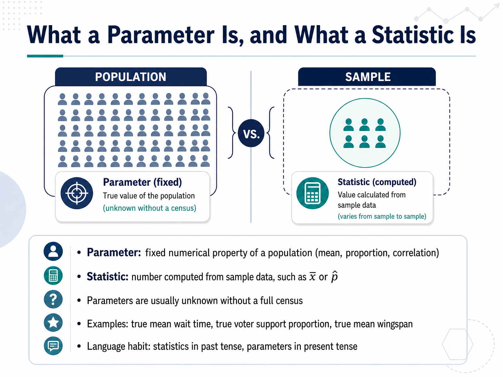
02What a Parameter Is, and What a Statistic IsLet's draw the key distinction. A parameter is a fixed numerical property of a population. For example, the true mean wait time for every customer at a service center is a parameter. A statistic is a number computed from sample data, such as the sample mean, written x bar, or the sample proportion, written p hat. Here is the core idea. Parameters are usually unknown without a full census. We rarely measure everyone, so the true voter support proportion or the true mean wingspan of a species stays hidden. Statistics, by contrast, are what we actually calculate from the data in front of us. One useful language habit. Use past tense for statistics, because they came from collected data. Use present tense for parameters, because they describe a fixed, ongoing truth. That small shift in wording keeps your reasoning precise. 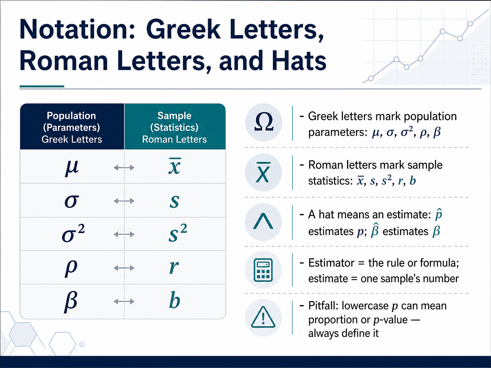Next, let's look at notation: Greek letters, Roman letters, and hats.1 min
03Notation: Greek Letters, Roman Letters, and HatsNow let's talk about notation, because the symbols tell you what kind of quantity you're looking at. Greek letters mark population parameters: mu, sigma, sigma squared, rho, and beta. Roman letters mark sample statistics: x bar, s, s squared, r, and b. So when you see sigma, think population. When you see s, think sample. Next, a hat means an estimate. For example, p hat estimates p, and beta hat estimates beta. Also keep two words separate in your mind. An estimator is the rule or formula. An estimate is one sample's number. Finally, a common pitfall: lowercase p can mean a proportion or a p-value, so always define it before you use it. With that notation in place, we can ask why parameters matter. 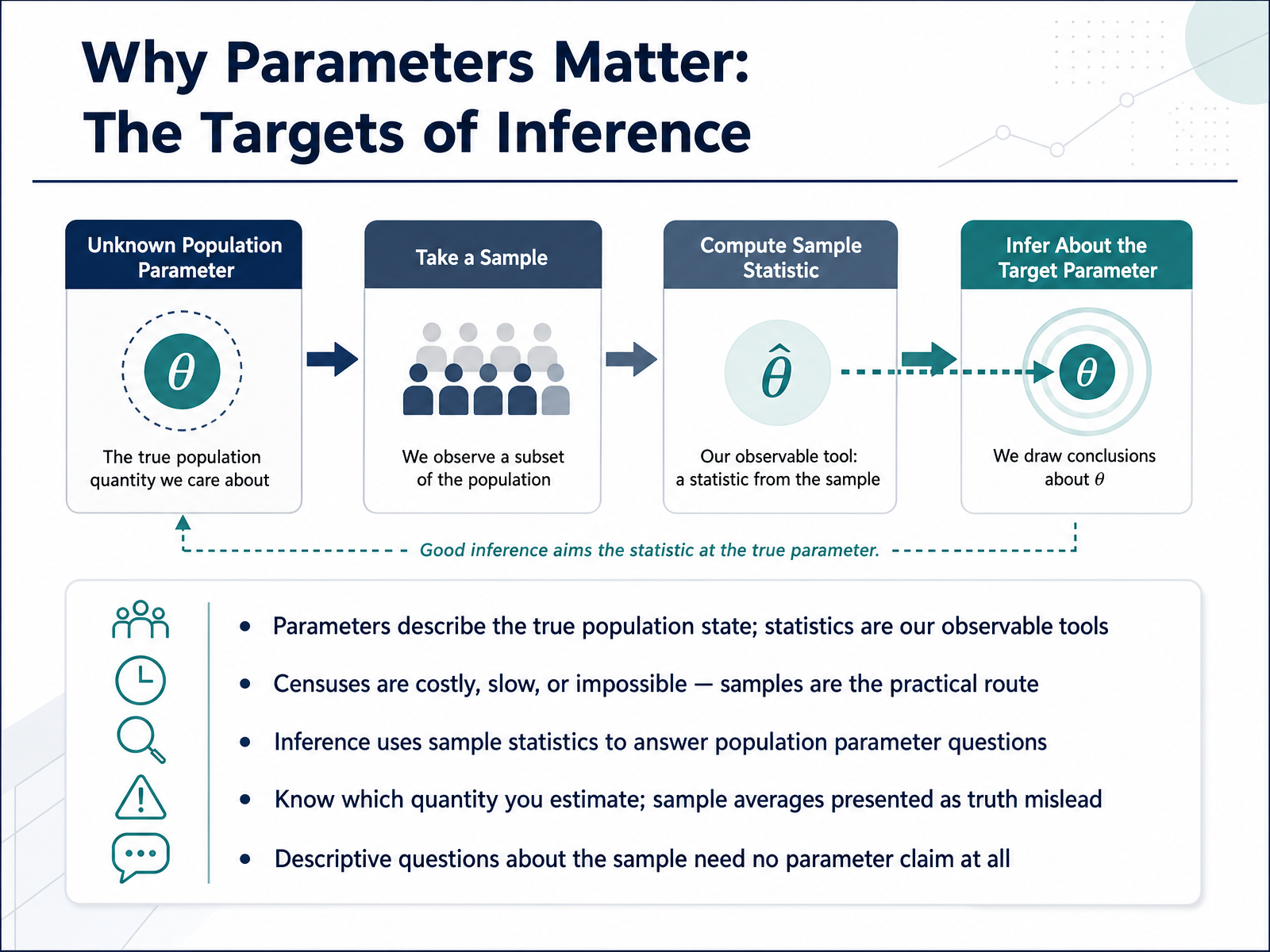They are the targets of inference.1 min
04Why Parameters Matter: The Targets of InferenceNow let's talk about why parameters matter. They are the targets of inference. A parameter describes the true state of a population, while a statistic is simply our observable tool, a number we can actually calculate from data we collect. In practice, a full census is often too costly, too slow, or even impossible. So we rely on samples as the practical route. Statistical inference uses sample statistics to answer questions about population parameters. For example, we might use a sample average to estimate a population mean. The key is to know exactly which quantity you are estimating. Presenting a sample average as if it were the truth can mislead your audience. And remember, if a question is purely descriptive about the sample itself, no parameter claim is needed at all. 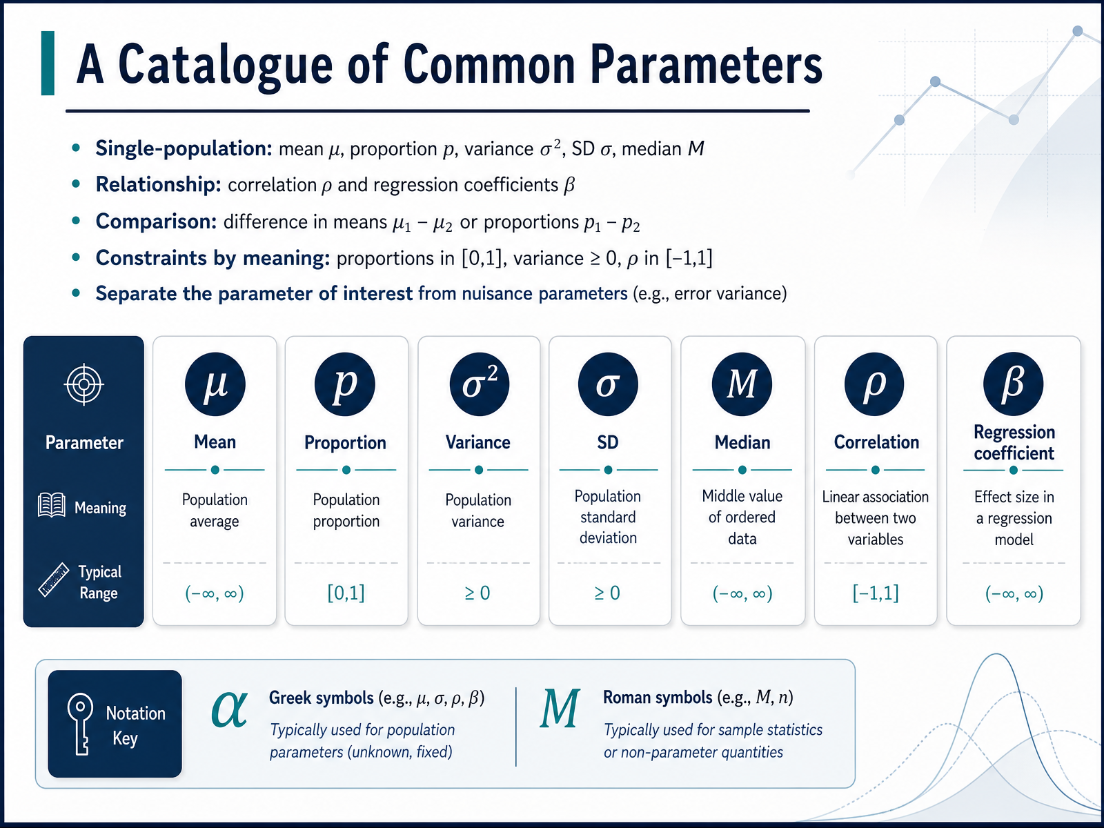Let's move on to a catalogue of common parameters.1 min
05A Catalogue of Common ParametersNow let's build a catalogue of common parameters. In a single population, the mean is mu, the proportion is p, the variance is sigma squared, the standard deviation is sigma, and the median is M. For relationships, we have the correlation, rho, and regression coefficients, beta. When comparing groups, the parameter might be the difference in means, mu one minus mu two, or the difference in proportions, p one minus p two. Each parameter also has constraints by meaning. A proportion must be between zero and one. A variance must be greater than or equal to zero. And a correlation must be between negative one and one. Finally, separate the parameter of interest from nuisance parameters. In a regression, beta is often the focus, while the error variance is a nuisance parameter. That distinction keeps your analysis targeted. Next, we will look at sampling variability, and why estimates differ.1 min
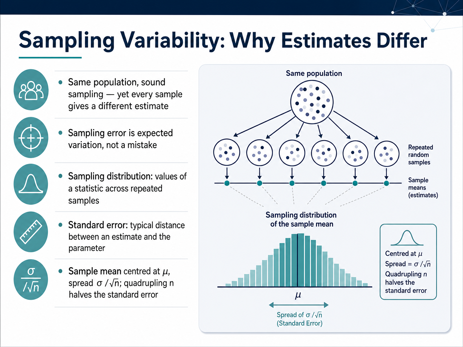
06Sampling Variability: Why Estimates DifferNow let's look at sampling variability, and why our estimates differ. Suppose you draw one random sample from a population, then another, then another. You use sound sampling every time. Yet each sample produces a different estimate. That is not a flaw in your method. It is expected variation, and we call it sampling error. Sampling error is not a mistake; it is natural variation. To describe it, we use the sampling distribution. That is the pattern of a statistic's values across many repeated samples. From that pattern, we get the standard error, which is the typical distance between an estimate and the true parameter. A small standard error means estimates cluster tightly around the truth. Here is a concrete case. For the sample mean, the sampling distribution is centred at mu, the population mean. Its spread is sigma divided by the square root of n, where n is the sample size. Notice the effect: quadrupling n halves the standard error. So more data means more precision. Takeaway: different samples give different estimates, and that is fine. The standard error tells you how much to trust any single one. 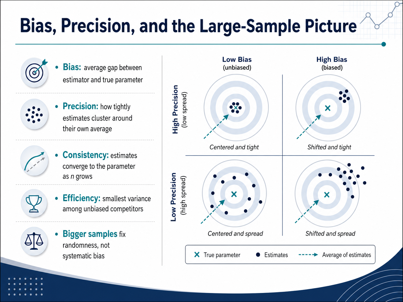Next, we move to the broader picture with bias, precision, and the large-sample view.2 min
07Bias, Precision, and the Large-Sample PictureLet us look at what makes one estimator better than another. Bias is the average gap between an estimator and the true parameter. Think of a scale that always reads two pounds heavy. That is bias, and it does not disappear just because you weigh more people. Precision is how tightly estimates cluster around their own average. A precise estimator gives similar values each time, even if they are slightly off target. Consistency means estimates converge to the parameter as sample size n grows. Efficiency means the estimator has the smallest variance among unbiased competitors. Here is the key takeaway. Bigger samples reduce randomness, so estimates become more stable. But bigger samples do not fix systematic bias. If your measurement tool is flawed, more data simply gives you a more confident wrong answer. So check both. Reduce random error with larger samples, and correct systematic error by improving how you measure or model. 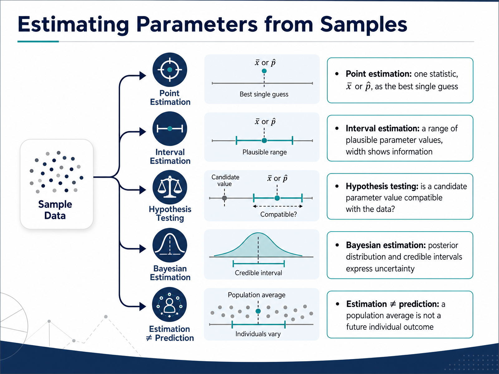Next, we will see how to put these ideas into practice in estimating parameters from samples.2 min
08Estimating Parameters from SamplesNow let's look at how we estimate parameters from samples. A point estimate uses one statistic, like the sample mean, x bar, or the sample proportion, p hat, as the best single guess for the population parameter. For example, if you survey one hundred customers and find an average satisfaction score of four point two, that is your point estimate. An interval estimate gives a range of plausible parameter values, and the width of that range shows how much information you have. A narrow interval means more precision. Hypothesis testing asks a different question: is a candidate parameter value compatible with the data? Bayesian estimation uses a posterior distribution and credible intervals to express uncertainty directly. Finally, remember that estimation is not prediction. A population average is not a future individual outcome. A store's average daily sales does not tell you exactly what tomorrow's sales will be. 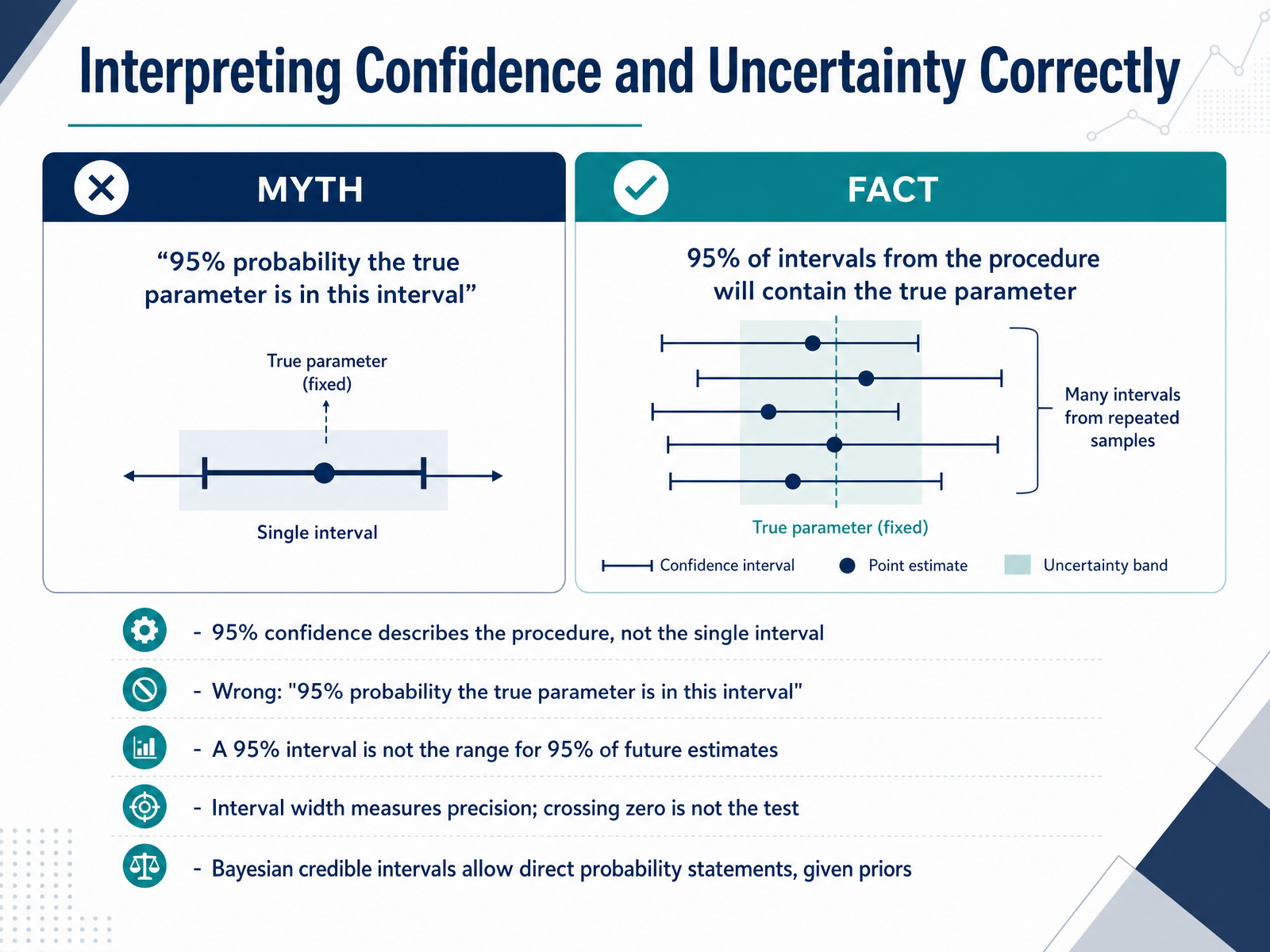Next, we will explore interpreting confidence and uncertainty correctly.2 min
09Interpreting Confidence and Uncertainty CorrectlyLet's tackle one of the most common mistakes in statistics: what confidence really means. A ninety five percent confidence level describes the procedure, not any single interval. If you repeated your sampling process many times, about ninety five percent of the intervals you build would capture the true parameter. So it is wrong to say there is a ninety five percent probability that the true parameter lies in this specific interval. The parameter is fixed, not random, so that probability statement does not apply. Also, a ninety five percent interval is not the range that contains ninety five percent of future estimates. That is a different idea. Instead, the width of the interval tells you about precision. A wider interval means less precision, and a narrower one means more. And do not fall for the trap of checking whether the interval crosses zero as a significance test. That is not what the interval is for. Now, if you want a direct probability statement about the parameter, you would need a Bayesian credible interval, which incorporates prior beliefs. That is a different framework. So the key takeaway is to interpret confidence as a property of your method, and use interval width to judge precision. 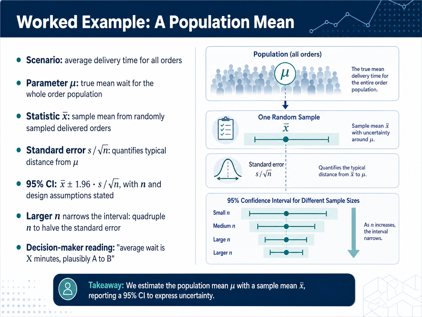Next, we will walk through a worked example involving a population mean.2 min
10Worked Example: A Population MeanLet's make the population mean concrete with a delivery-time example. Suppose a company wants to understand the average wait for all of its orders. The parameter mu is the true mean wait across the entire order population. That value is fixed, but usually unknown. The statistic x-bar is the sample mean, computed from randomly sampled delivered orders. It estimates mu. Because samples vary, we report a standard error, s divided by the square root of n. That value quantifies the typical distance between x-bar and mu. A ninety-five percent confidence interval is x-bar plus or minus one point nine six times s divided by the square root of n, with n and design assumptions stated. Larger samples narrow the interval. In fact, quadrupling n halves the standard error. A decision-maker can then read it plainly: the average wait is X minutes, plausibly between A and B. That is how a parameter becomes a useful decision tool. 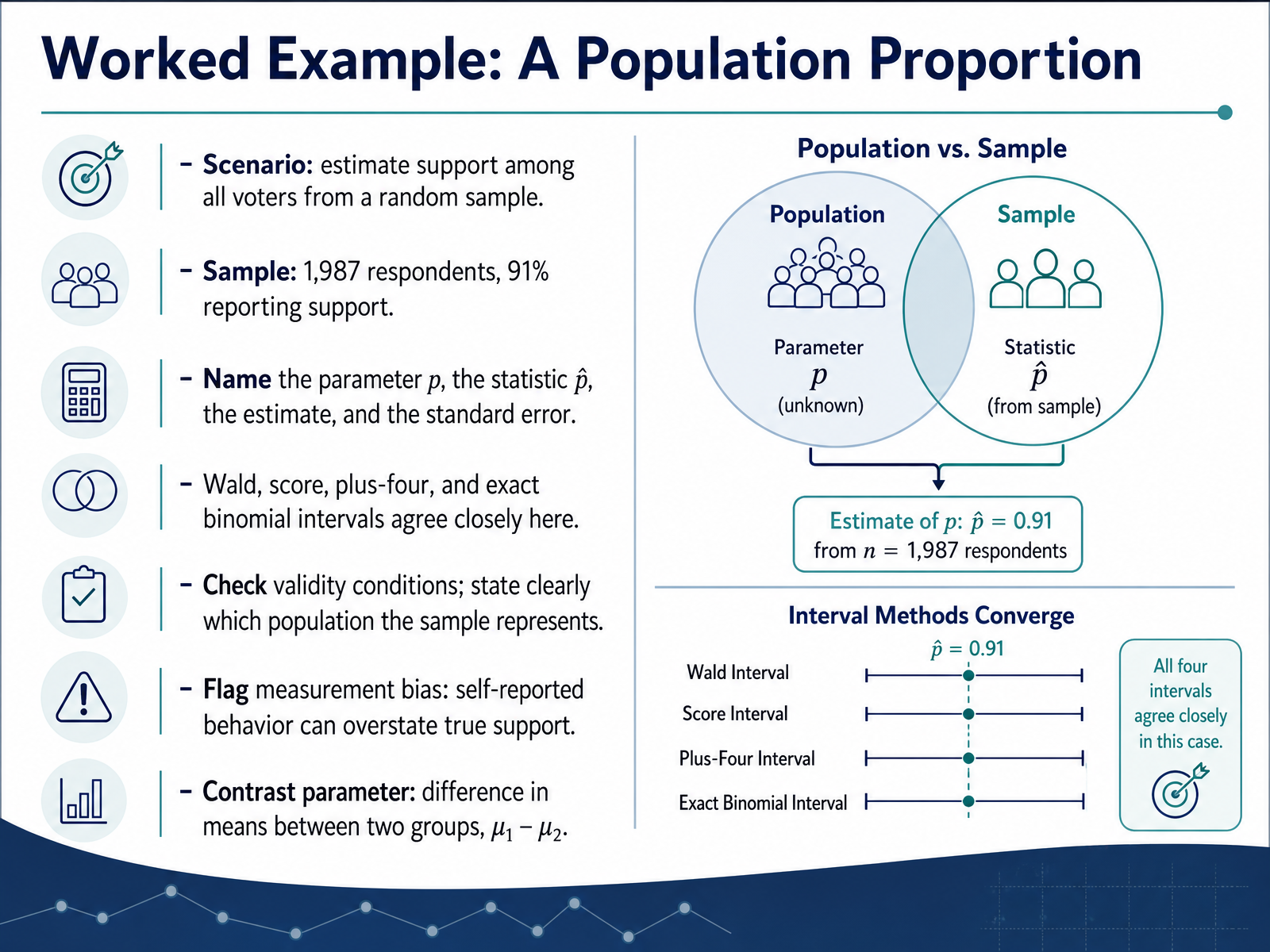Next, we will work through a population proportion.2 min
11Worked Example: A Population ProportionNow let's work through a concrete example using a population proportion. Suppose you want to estimate support among all voters in a city. You draw a random sample of one thousand nine hundred eighty-seven respondents, and ninety-one percent report support. The parameter, written p, is the true proportion of support in the entire voter population. The statistic, written p hat, is the ninety-one percent you observed in the sample. Your estimate of p is zero point nine one, and the standard error tells you how much that estimate would vary from sample to sample. With this sample size, the Wald, score, plus-four, and exact binomial intervals agree closely, so your conclusion is stable across methods. Still, check two things. First, validity conditions: is the sample random and large enough? Second, define the population carefully. Which voters does this represent? Also flag measurement bias. Self-reported support often overstates real behavior. Finally, compare this to another parameter. Instead of a single proportion, you might study the difference in means between two groups, mu one minus mu two. 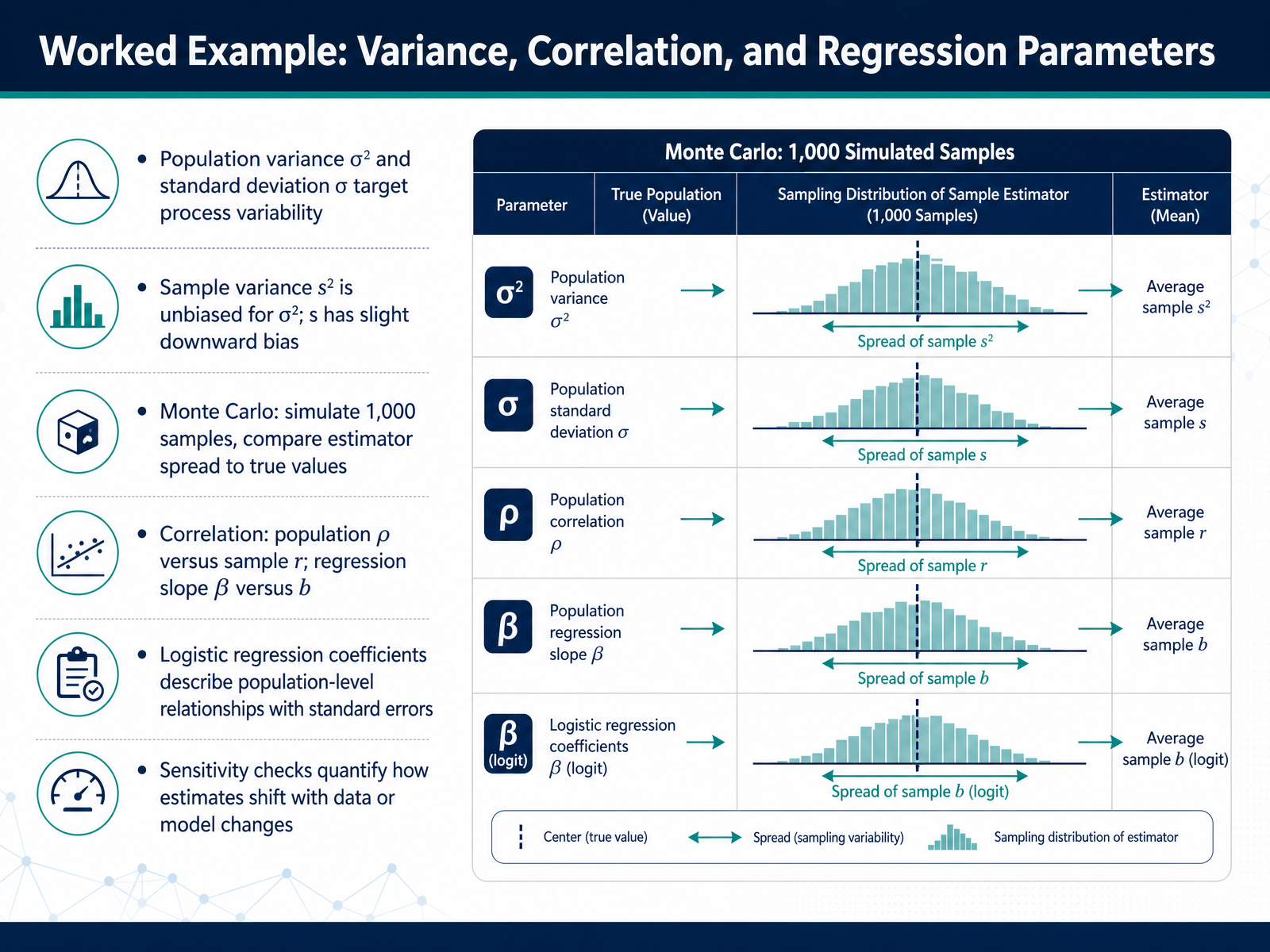Next, we move to variance, correlation, and regression parameters.2 min
12Worked Example: Variance, Correlation, and Regression ParametersLet's work through a concrete example that ties variance, correlation, and regression parameters together. Suppose you monitor a manufacturing process. The population variance, written sigma squared, and the population standard deviation, sigma, describe the true variability of that process over all time. In practice, you only have a sample, so you calculate the sample variance, s squared, which is unbiased for sigma squared. The sample standard deviation, s, however, has a slight downward bias, meaning it tends to underestimate the true spread just a little. To see this clearly, you can run a Monte Carlo simulation. Simulate one thousand samples, and compare the spread of your estimates to the true values. That shows you how much sampling error to expect. Next, think about relationships. The population correlation, rho, measures the true linear association between two variables. The sample correlation, r, estimates it. In regression, the population slope, beta, is the true average change in the outcome for a one unit change in the predictor. The sample slope, b, estimates that. For logistic regression, the coefficients describe population level relationships on the log odds scale, and their standard errors tell you how precise those estimates are. Finally, sensitivity checks quantify how much your estimates shift when you change the data or the model. That helps you judge robustness. 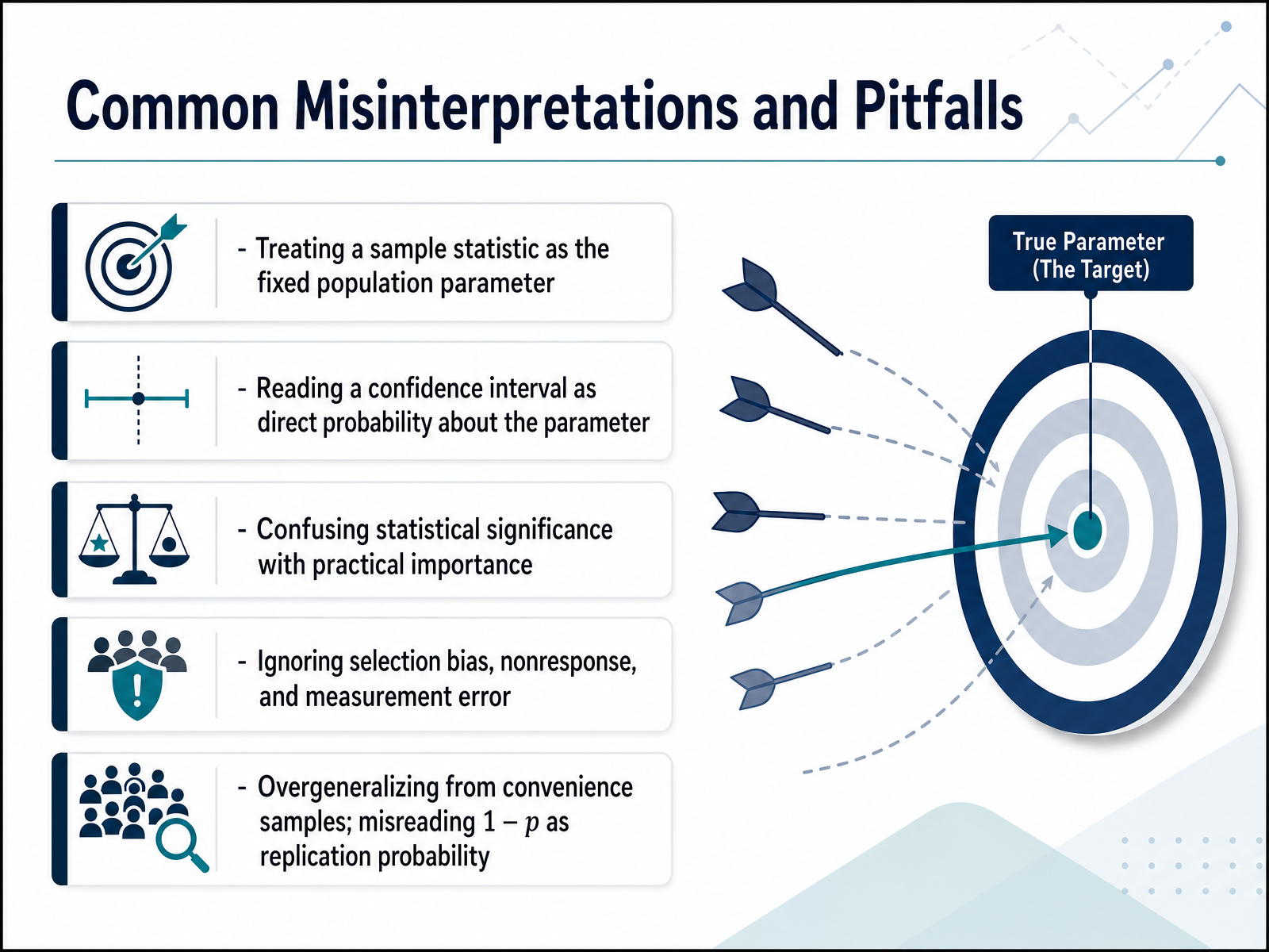As we move on, we'll look at common misinterpretations and pitfalls, so you can avoid them in your own work.2 min
13Common Misinterpretations and PitfallsLet's turn to the common misinterpretations and pitfalls you should watch for. First, treating a sample statistic as the fixed population parameter. A sample mean is an estimate, not the truth. It varies from sample to sample, while the parameter is fixed but usually unknown. Second, reading a confidence interval as a direct probability about the parameter. A ninety-five percent confidence interval means the method captures the parameter in ninety-five percent of repeated samples, not that there is a ninety-five percent chance the parameter falls inside this one interval. Third, confusing statistical significance with practical importance. A tiny effect can be significant with a large sample, yet matter little in real decisions. Fourth, ignoring selection bias, nonresponse, and measurement error. If your sample systematically excludes part of the population, your estimate is distorted no matter how large it is. Fifth, overgeneralizing from convenience samples, and misreading one minus p as the probability of replication. A small p value does not tell you how likely a study is to repeat. In short, always ask how the data were collected, what uncertainty means, and whether the difference matters. 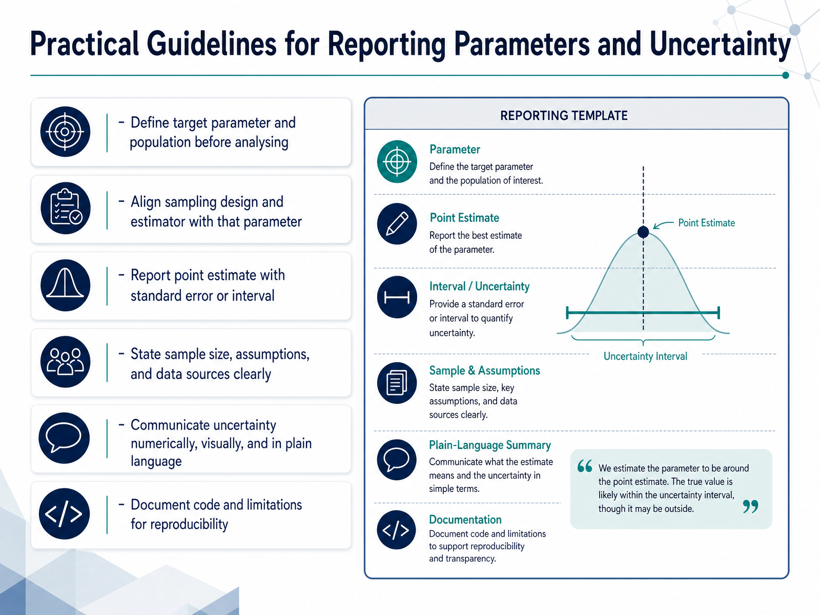Let's move on to practical guidelines for reporting parameters and uncertainty.2 min
14Practical Guidelines for Reporting Parameters and UncertaintyLet's turn these ideas into practical guidelines you can apply whenever you report a parameter. First, before you analyze anything, define your target parameter and the population it describes. For example, decide whether you want the average income of all small businesses in a city, not just the ones in your survey. Next, align your sampling design and your estimator with that parameter. If you want a total, use an estimator for a total, not for a mean. When you report results, always give a point estimate together with a measure of uncertainty, such as a standard error or a confidence interval. Then state the sample size, the assumptions you made, and where the data came from. Communicate uncertainty in three ways: numerically, visually, and in plain language, like saying the estimate is about forty thousand dollars, give or take three thousand. Finally, document your code and note the limitations, so others can reproduce your work. Keep this checklist handy, and your parameter reports will be clear, honest, and useful. 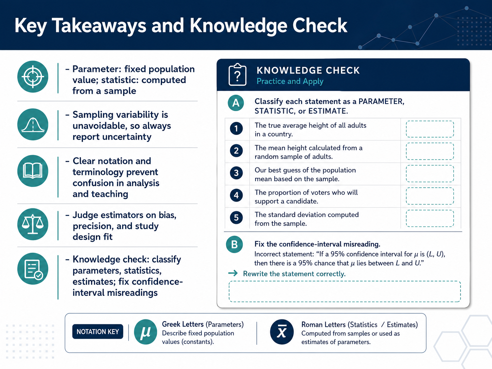That prepares us for our final segment: Key Takeaways and Knowledge Check.2 min
15Key Takeaways and Knowledge CheckLet's bring it all together. A parameter is a fixed value for the whole population. A statistic is computed from a sample. So the population mean is a parameter, while your sample mean is a statistic. Because samples vary, sampling variability is unavoidable. Always report uncertainty, for example, a confidence interval rather than a single number. Clear notation and terminology prevent confusion, whether you are analyzing data or teaching a class. And judge estimators on bias, precision, and how well the study design fits the question. Now try the knowledge check. Classify each value as a parameter, a statistic, or an estimate. Then correct any misreadings of confidence intervals, such as saying there is a ninety-five percent chance the true value lies in this specific interval. Thank you for working through this course. Keep asking where the number came from, and you will make stronger, more honest decisions with data. Well done, and good luck in your next analysis.2 min

Take the deck with you

Download this course as a file — free, no sign-up needed.

PDF handoutEvery slide page, ready to print or share.16 pages · 4.0 MBDownload
Narrated PowerPointThe deck that presents itself — every slide carries the digital human's narration video.16 pages · 16.0 MBDownload
PowerPoint slidesThe full deck as a .pptx — open it in PowerPoint, Keynote, or Google Slides.16 pages · 3.8 MBDownload

Free to use in your own training — please keep the PersonWise credit page at the end.

Have your own deck? Turn it into a course

Sources consulted

Web sources consulted while building this course.