Digital Signal Processing Fundamentals

Name: Digital Signal Processing Fundamentals
Availability: InStock

Learn the fundamentals of Digital Signal Processing, covering key concepts and applications for engineers and technical professionals.

My workspace30 minFree to watch

What you’ll learn

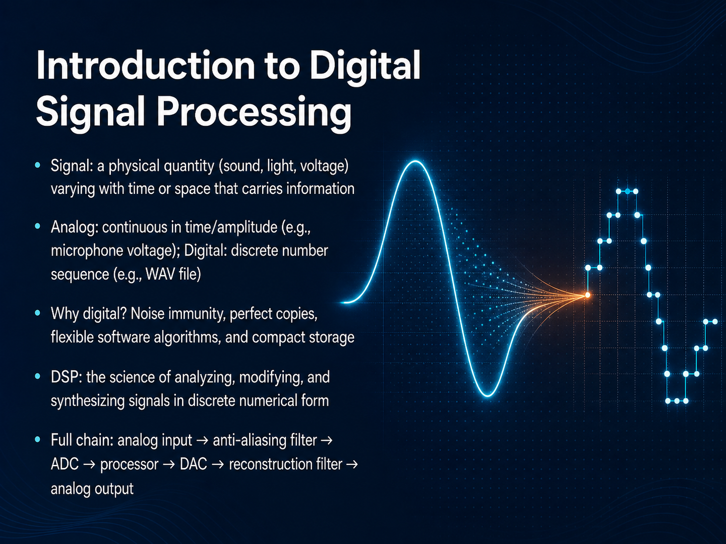
01Introduction to Digital Signal ProcessingWelcome. In this course we explore digital signal processing, or DSP, and how it transforms real-world information into precise, flexible data. Let us start with the core idea. A signal is any physical quantity that changes over time or space and carries information. Sound, light, and voltage are everyday examples. In the analog world, signals are continuous in both time and amplitude, like the voltage from a microphone. Digital signals are different. They consist of discrete number sequences, much like the data inside a WAV file. So why go digital? The benefits are powerful. Digital systems resist noise, produce perfect copies, run flexible software algorithms, and enable compact storage. DSP is the science behind this conversion. It analyzes, modifies, and synthesizes signals using numerical techniques. The full chain moves from an analog input through an anti-aliasing filter and an analog-to-digital converter. The processor then performs the DSP operations. After processing, a digital-to-analog converter and a reconstruction filter return the signal to the analog world. This journey from continuous waves to discrete numbers and back is the foundation of everything we will cover, from audio compression to medical imaging. Next we will look at how this digital magic powers everyday devices in the slide, Why Go Digital? Everyday Magic Powered by DSP.doi.org nature.com link.springer.com+22 min
02Why Go Digital? Everyday Magic Powered by DSPMoving from that big picture, let's ground this in the technology you already use every day. When you stream a song, the music exists as a stream of numbers, not a fragile magnetic tape. That digital file can be copied infinitely with zero degradation. Noise-canceling headphones are essentially tiny DSP systems analyzing ambient sound and generating inverse waves in real time. Voice assistants, too, wake up by constantly running lightweight neural keyword spotting directly on device hardware. The beauty of DSP is that the same physical chip can become entirely different instruments through software alone: a guitar pedal, a medical monitor, or a radar processor. This is what enables on-device AI to run person detection or keyword spotting using only milliwatts of power, often harvested from ambient light. This entire chain of sampling, representing, and filtering signals is what powers wireless communication, biomedical imaging, and the audio codecs behind every call and track you hear. Next, we will take the first step into the actual process: sampling, which means capturing the continuous world as a series of snapshots.doi.org nature.com link.springer.com+22 min
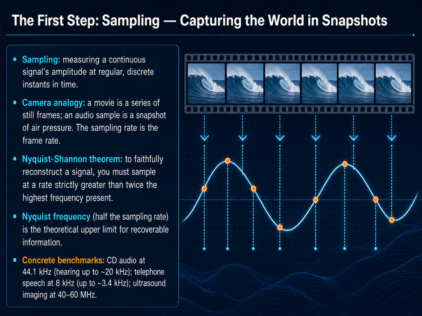
03The First Step: Sampling — Capturing the World in SnapshotsNow let’s focus on the first step: sampling. Think of sampling as capturing the real world in snapshots. Instead of tracking a continuous signal perfectly, we measure its amplitude at regular, discrete instants in time. A familiar analogy is video. A movie isn’t true motion; it’s a series of still frames played quickly. Audio sampling works the same way. Each sample is a snapshot of air pressure at a precise moment, and the sampling rate acts like the frame rate. The higher the rate, the more snapshots we take. The rule that governs all of this is the Nyquist-Shannon theorem. To faithfully reconstruct a signal, you must sample at a rate strictly greater than twice the highest frequency present. Half the sampling rate is called the Nyquist frequency, and it represents the theoretical upper limit for recoverable information. Concrete benchmarks make this clear. CD audio uses forty-four point one kilohertz, which covers human hearing up to about twenty kilohertz with a small guard band. Telephone speech, designed only for intelligibility, samples at eight kilohertz to capture frequencies up to roughly three point four kilohertz. At the other extreme, ultrasound imaging operates at forty to sixty megahertz to capture extremely high-frequency sound waves. Next, we will explore what happens when we ignore these limits, as we look at the specter of undersampling and introduce aliasing.cursa.app thoughtfulexaminations.com medium.com+22 min
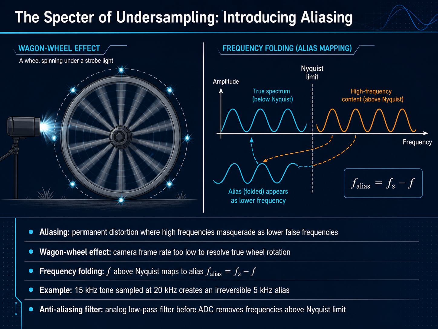
04The Specter of Undersampling: Introducing AliasingNow let's confront one of the most important challenges in digital signal processing: aliasing. Aliasing is a permanent distortion that happens when we sample too slowly. High frequencies don't just disappear. They disguise themselves as lower, completely false frequencies in your digital data. Think of the wagon-wheel effect in movies. When a camera's frame rate is too low to capture the true rotation speed, the wheel appears to spin backward or at the wrong speed. The same thing happens when you digitize an audio tone. Imagine a 15 kilohertz tone sampled at only 20 kilohertz. Because we are sampling below the Nyquist rate, the system can't track the true cycles. It incorrectly reconstructs a 5 kilohertz alias. Once that alias is in the data, you cannot remove it. It is indistinguishable from a real 5 kilohertz signal. To prevent this, we use an anti-aliasing filter. This is an analog low-pass filter placed before the ADC. It removes any frequencies above the Nyquist limit before they can cause problems. With the hazards of sampling established, our next step is to look at how these clean samples get converted into digital numbers. Up next: Bit by Bit: Quantization and the Staircase of Precision.cursa.app thoughtfulexaminations.com medium.com+22 min
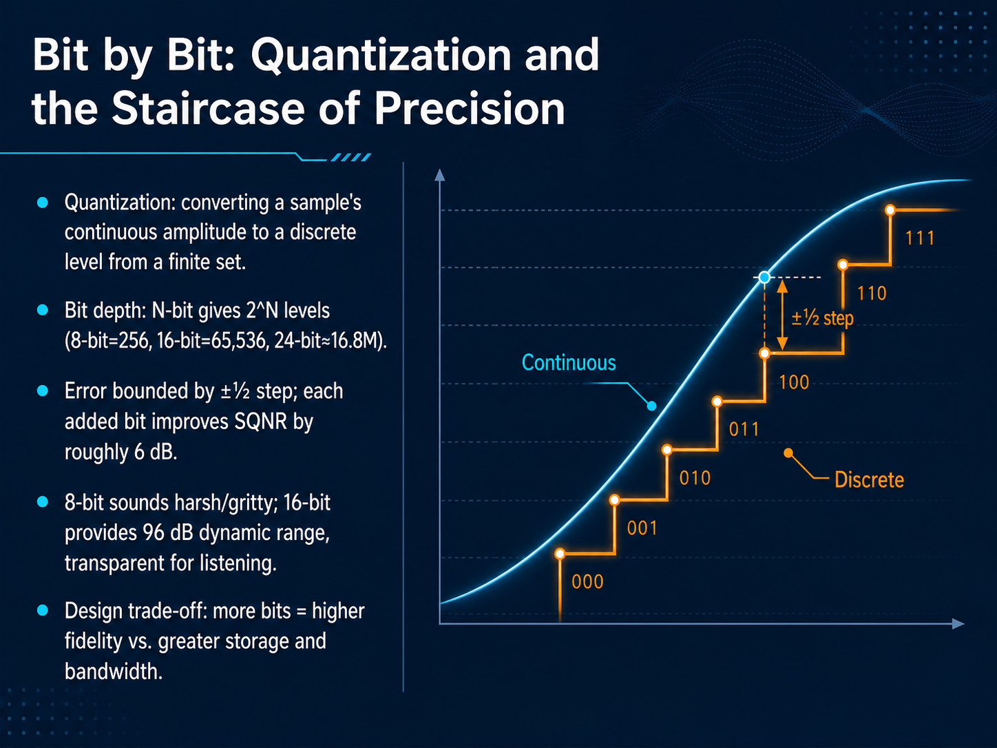
05Bit by Bit: Quantization and the Staircase of PrecisionNow let's get precise about the third step: quantization. After sampling captures the signal's value at a moment in time, we need to convert that continuous amplitude into a discrete level from a finite set. This process is what we call quantization, and it's a bit like rounding. Imagine a staircase: no matter where you place your foot on a step, its final recorded height is the single value of that step. A sample's true amplitude is forced to the nearest available level, creating a small amount of error. We call this error quantization noise. The number of bits we use defines how many steps we have. An N-bit system gives us two to the power of N levels. For example, 8-bit audio provides only 256 levels. This low resolution sounds harsh and gritty because the error between the true signal and the quantized value is relatively large. By contrast, 16-bit audio gives us sixty-five thousand five hundred thirty-six levels, which pushes the quantization noise down to about ninety-six decibels below the signal. In practical terms, that noise floor is so low it's transparent for listening. Each added bit improves the signal-to-quantization-noise ratio by roughly six decibels. The trade-off is clear: more bits mean higher fidelity but also require greater storage and bandwidth. Next, we'll see how these discrete samples form a sequence, moving us into discrete-time operations.dspillustrations.com tonestack.net audiocheck.net+22 min
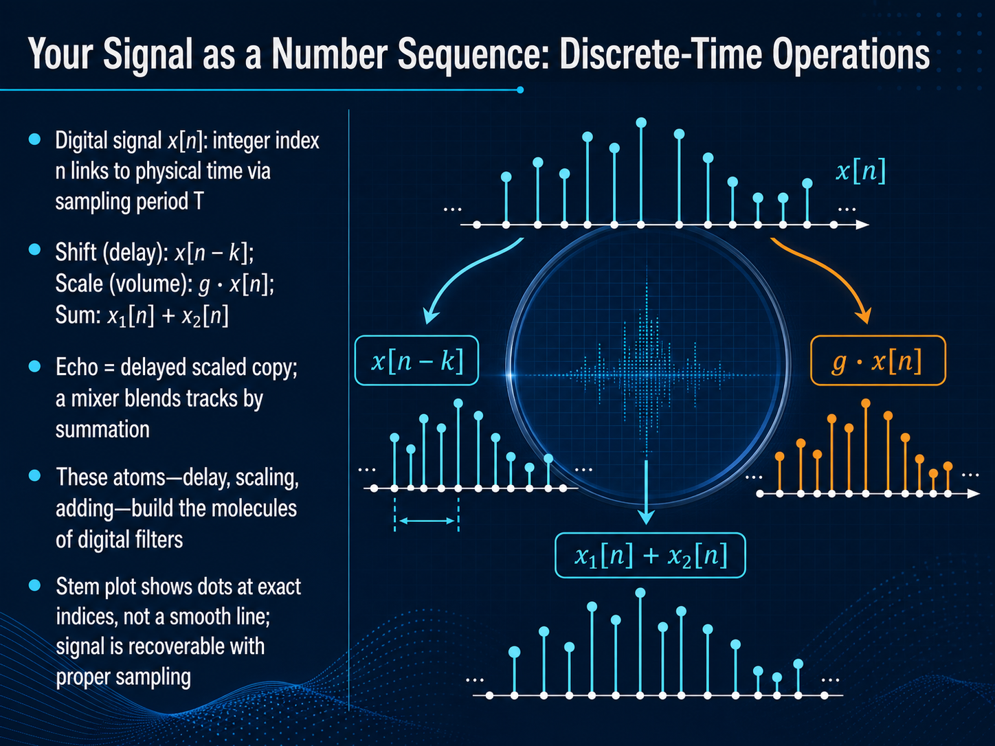
06Your Signal as a Number Sequence: Discrete-Time OperationsNow let's look at what your sampled signal actually becomes in the computer: a sequence of numbers. We write it as x of n, where the integer index n links back to real physical time through the sampling period T. Once you have this sequence, you can start doing useful operations. The three fundamental ones are shift, which is just a delay written as x of n minus k; scale, which changes the volume by multiplying by a factor g; and sum, which adds two sequences sample by sample. These simple building blocks are more powerful than they look. For example, when you delay a signal and scale it down, then add it to the original, you have created an echo. If you add two different tracks together, you are building a mixer. These atoms of delay, scaling, and adding become the molecules that make up all digital filters. On a stem plot, a digital signal looks like a series of dots at exact sample indices. It is not a smooth continuous line. That is an important visual habit to form. As long as you followed proper sampling rules, the original continuous signal is fully recoverable from exactly these dots. Coming up next, we will see one of the simplest and most intuitive realizations of these operations: gentle smoothing with the moving-average filter.compoundlearn.ai schaumont.dyn.wpi.edu schaumont.dyn.wpi.edu+22 min
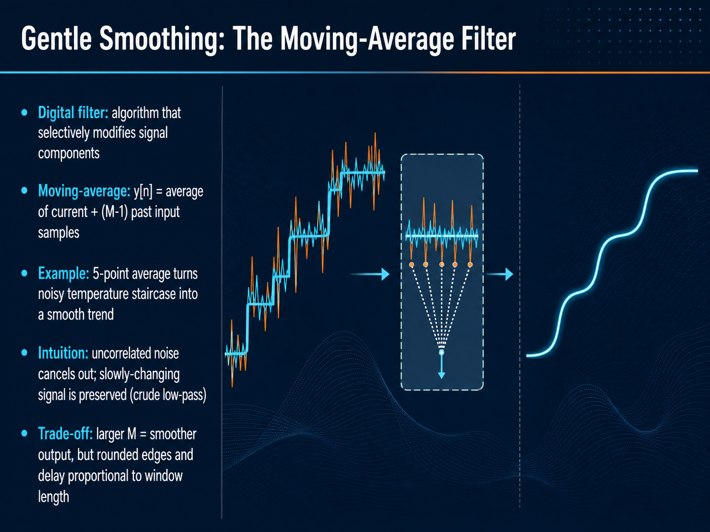
07Gentle Smoothing: The Moving-Average FilterLet's start putting these concepts into practice with one of the simplest and most widely used digital filters. It's called the moving-average filter, and it's a perfect introduction to gentle signal smoothing. Think of it as an algorithm that selectively modifies your signal components. The idea is straightforward: for every output point y of n, you simply average the current input sample together with a fixed number, M minus 1, of the most recent past samples. For example, a 5-point moving average would take your noisy temperature reading plus the four readings just before it and compute their mean. This works because random, uncorrelated noise tends to cancel itself out when you average multiple samples, while the slowly changing underlying temperature trend is preserved. In signal processing terms, this gives you a crude but effective low-pass filter. The intuition is clear: the filter smooths out rapid, random fluctuations while letting the persistent signal through. However, there is a fundamental trade-off. Choosing a larger M, a wider window, gives you an even smoother output with less noise, but it also rounds off sharp edges in your signal and introduces a delay. That delay is roughly proportional to the length of your averaging window, so there's always a balance. Next, we'll build on this foundation and explore FIR filters, which use weighted sums of past and present samples to create more precise shaping.cursa.app thoughtfulexaminations.com medium.com+22 min
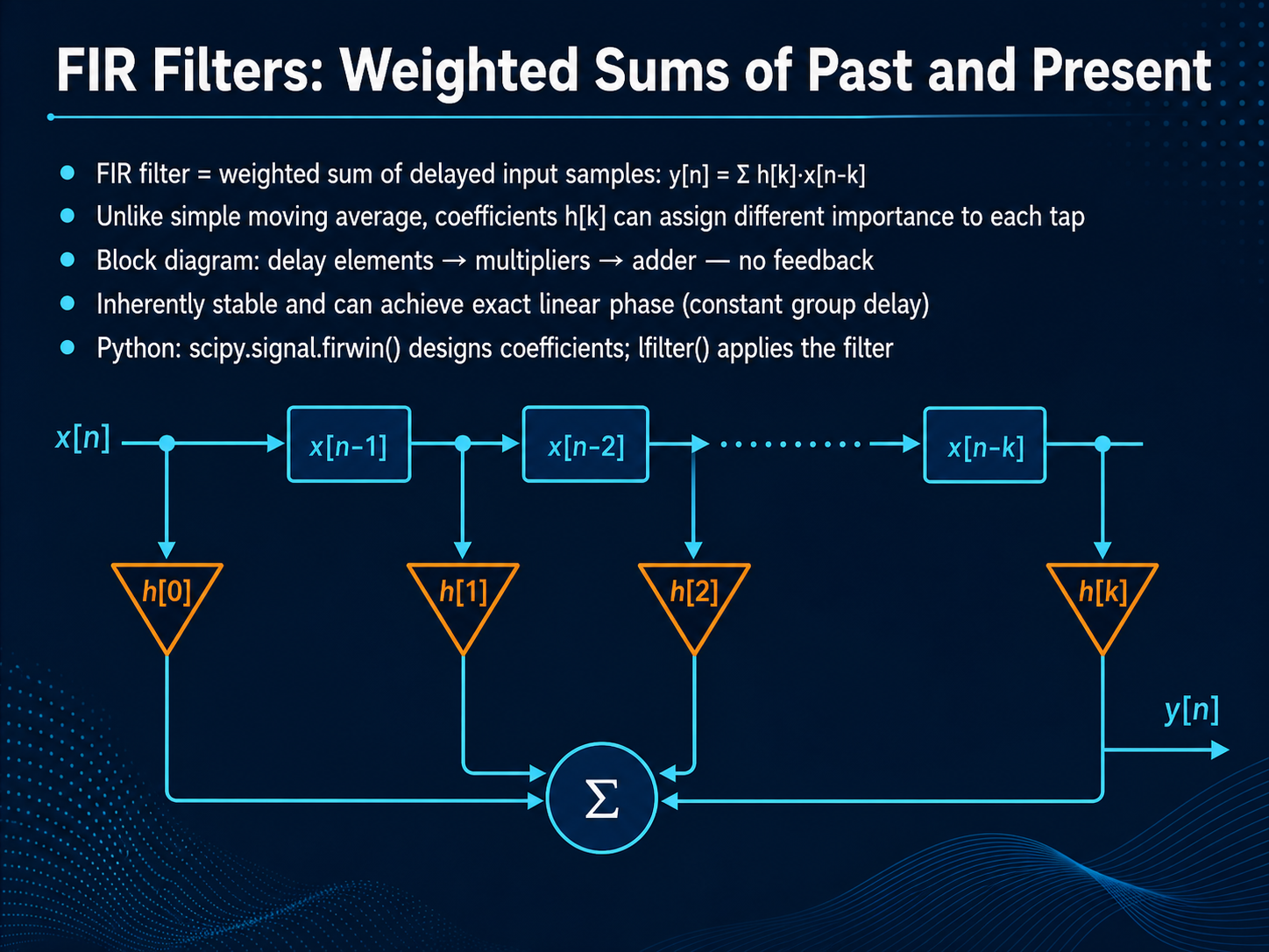
08FIR Filters: Weighted Sums of Past and PresentNow we turn to the FIR filter, which is fundamentally a weighted sum of delayed input samples. The output at any moment is a combination of the current sample and a finite set of past samples, each multiplied by its own coefficient. Unlike a simple moving average where every point gets equal weight, here we can assign different importance to each tap. That flexibility is what lets us shape the frequency response precisely. If you look at the block diagram, the signal flows through delay elements, then multipliers, and finally into an adder. There is no feedback path at all. This structure is inherently stable, and it can achieve exact linear phase, meaning constant group delay. All frequency components pass through with the same delay. In Python, you can design the coefficients with scipy.signal.firwin, and apply the filter using lfilter. Next, we'll move into Seeing the Unseen: Time and Frequency Perspectives on Filtering.compoundlearn.ai schaumont.dyn.wpi.edu schaumont.dyn.wpi.edu+21 min
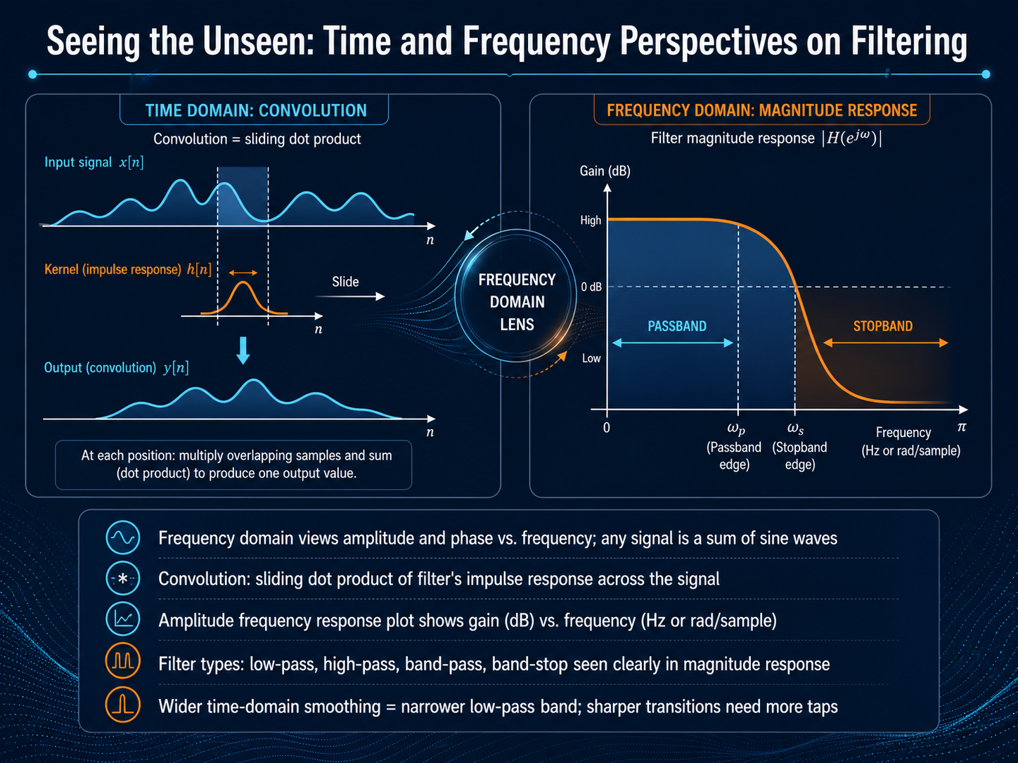
09Seeing the Unseen: Time and Frequency Perspectives on FilteringNow we shift our perspective to see what filtering looks like in the frequency domain. Think of any signal, such as an audio recording, as a sum of sine waves. The frequency domain view plots the amplitude and phase of those sine waves against frequency. Filtering means we reshape this spectrum. We do this through convolution. In simple terms, convolution slides the filter's impulse response across the signal, computing a weighted dot product at each step. This operation shapes which sine waves pass through and which get suppressed. You will often see this displayed as an amplitude frequency response plot, with gain in decibels on the vertical axis and frequency in hertz on the horizontal axis. This plot makes the classic filter types instantly recognizable. A low-pass filter shows a flat passband that transitions to a falling stopband. A high-pass filter rises from a suppressed low end. Band-pass filters isolate a middle region, and band-stop filters carve out a notch. There is also a direct link between the time and frequency domains. Wider time smoothing, which means averaging over more samples, produces a narrower low-pass band with a softer transition. If you need a sharper transition, you must use more filter taps or a higher order. 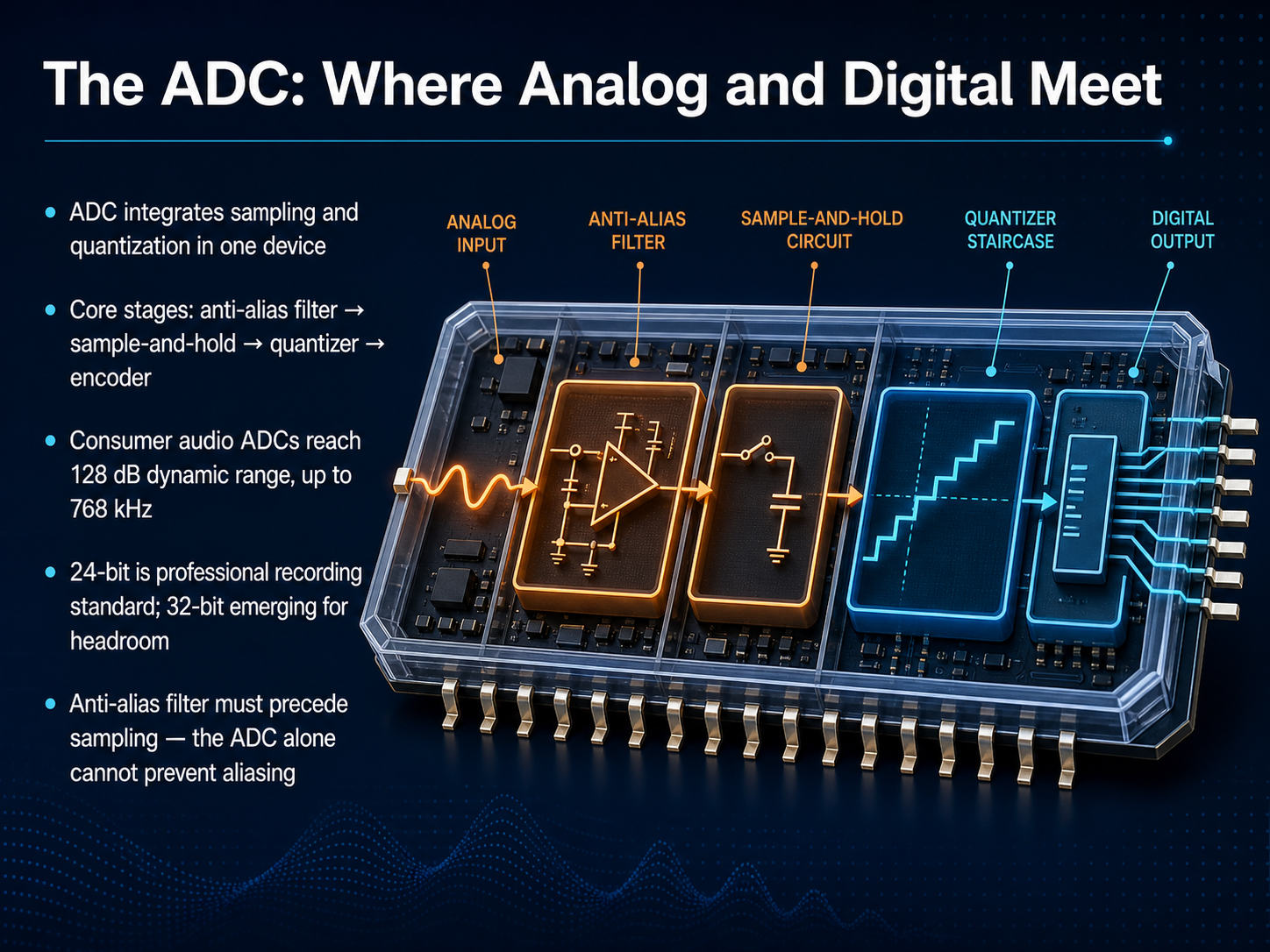Next, we will look at how these digital concepts connect back to the physical world in The ADC: Where Analog and Digital Meet.2 min
10The ADC: Where Analog and Digital MeetNow, let's bring these concepts together inside a single physical device: the analog-to-digital converter, or ADC. This is the critical bridge where a continuous analog signal, like the voltage from a microphone, becomes a stream of digital numbers. Internally, the ADC integrates both sampling and quantization in a carefully ordered sequence. The signal first passes through an anti-alias filter—a crucial step we must emphasize. This filter must come before sampling. The ADC alone cannot prevent aliasing; it simply digitizes whatever it receives, including any frequencies that would fold back and create false signals. Only by removing those frequencies with the analog anti-alias filter do we ensure a clean conversion. Next, the sample-and-hold stage captures the waveform's instantaneous voltage and holds it steady for the quantizer. The quantizer maps this voltage to the nearest discrete level, and the encoder outputs the final binary code. To put this in context, modern consumer audio ADCs can achieve an extraordinary 128 decibels of dynamic range and support sample rates up to 768 kilohertz. In professional recording, 24-bit depth is the absolute standard, providing a noise floor far below the signal. An emerging trend is 32-bit recording, which provides immense digital headroom, making it practically impossible to clip the signal during capture. As we move forward, we will see how the reverse process, the DAC, reconstructs the analog world from these precise digital codes.compoundlearn.ai schaumont.dyn.wpi.edu schaumont.dyn.wpi.edu+22 min
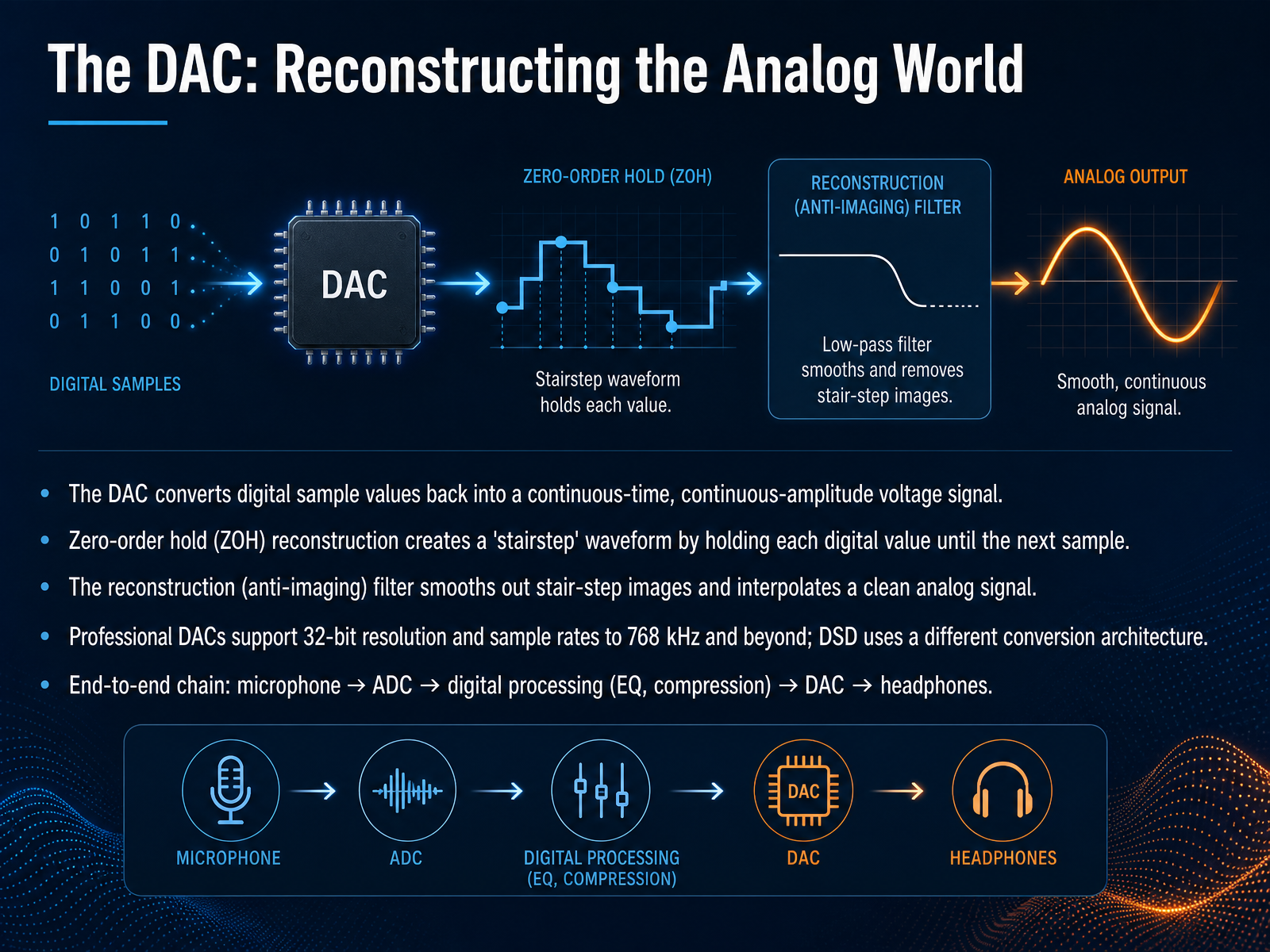
11The DAC: Reconstructing the Analog WorldNow let's bring the signal back to the continuous world. The digital-to-analog converter, or DAC, is the device that turns our processed digital samples into a smooth, continuous voltage signal we can actually hear or measure. The most basic reconstruction method is called zero-order hold. It simply holds each digital value steady until the next sample arrives, creating a waveform that looks like a staircase. That stairstep shape introduces high-frequency artifacts, often called images. To fix this, we use a reconstruction filter, sometimes called an anti-imaging filter. This analog filter smooths out the sharp steps and interpolates a clean, band-limited waveform. Professional DACs today are incredibly precise, often supporting 32-bit resolution and sample rates reaching 768 kilohertz or even higher. Some converters, like those using DSD, employ a completely different noise-shaping architecture. So to visualize the complete journey, think of a singer’s voice: the microphone captures the analog wave, the ADC samples and quantizes it, our digital processing applies EQ and compression, and then the DAC with its reconstruction filter drives your headphones with a clean analog signal. Next, we’ll explore what can go wrong in practice, including quantization, overflow, and instability.compoundlearn.ai schaumont.dyn.wpi.edu schaumont.dyn.wpi.edu+22 min
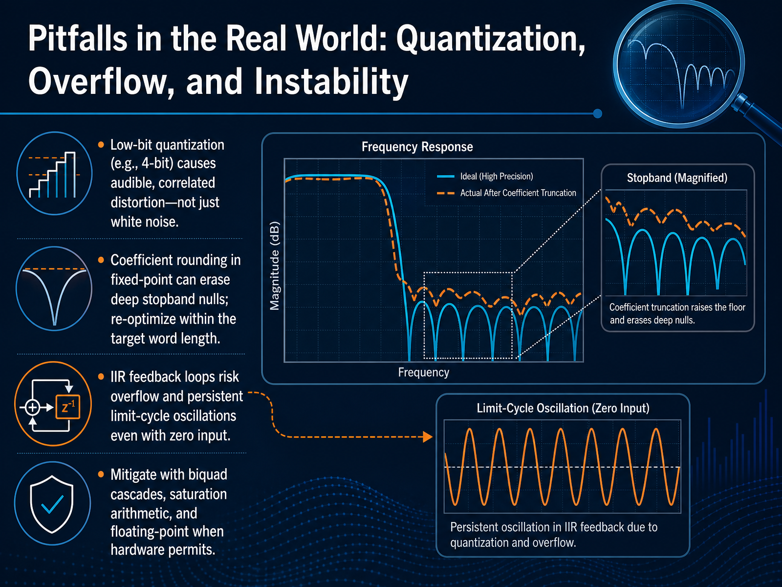
12Pitfalls in the Real World: Quantization, Overflow, and InstabilityNow let's look at some real world pitfalls you will face during implementation, specifically quantization, overflow, and instability. First, low bit quantization does not just add simple white noise. At four bits, for example, the distortion is audible and correlated to the signal itself, which sounds much worse than a gentle hiss. Next, when you round coefficients in fixed point designs, deep stopband nulls can completely disappear. To avoid this, you must re optimize your coefficients within your target word length. Another critical trap is the IIR feedback loop. Even with zero input, rounding errors can circulate and create persistent limit cycle oscillations. This can overflow and saturate your output. To mitigate these risks, switch to cascaded biquad sections instead of a single high order direct form. Always use saturation arithmetic to handle overflow gracefully, and if your hardware supports it, use floating point math to ease dynamic range constraints. Coming up next, we will explore DSP in action across audio, images, and biomedicine.dspillustrations.com tonestack.net audiocheck.net+22 min
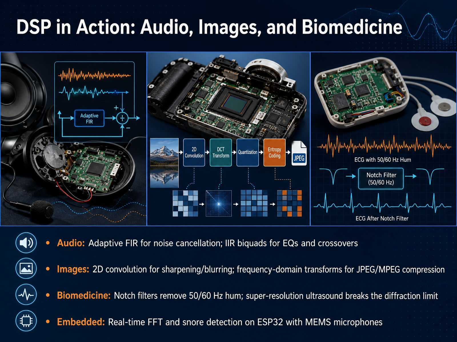
13DSP in Action: Audio, Images, and BiomedicineNow let's see digital signal processing in action across a few key fields. In audio, adaptive FIR filters enable real-time noise cancellation, while IIR biquad structures form the core of equalizers and crossovers you find in music production. In imaging, two-dimensional convolution handles sharpening and blurring, and frequency-domain transforms like the discrete cosine transform make JPEG and MPEG compression possible. Shifting to biomedicine, notch filters precisely remove fifty- or sixty-hertz power-line hum from physiological recordings. Researchers also use super-resolution ultrasound techniques to visualize microvascular details beyond the conventional diffraction limit. On the embedded side, real-time FFT running on an ESP32 with MEMS microphones can detect snoring patterns and estimate sleep apnea severity from a compact, low-power device. These applications all rely on the same fundamental principles of sampling, representation, and filtering. Next, we will shrink the scale even further: into the tiny world of DSP on microcontrollers and edge AI.doi.org nature.com link.springer.com+22 min
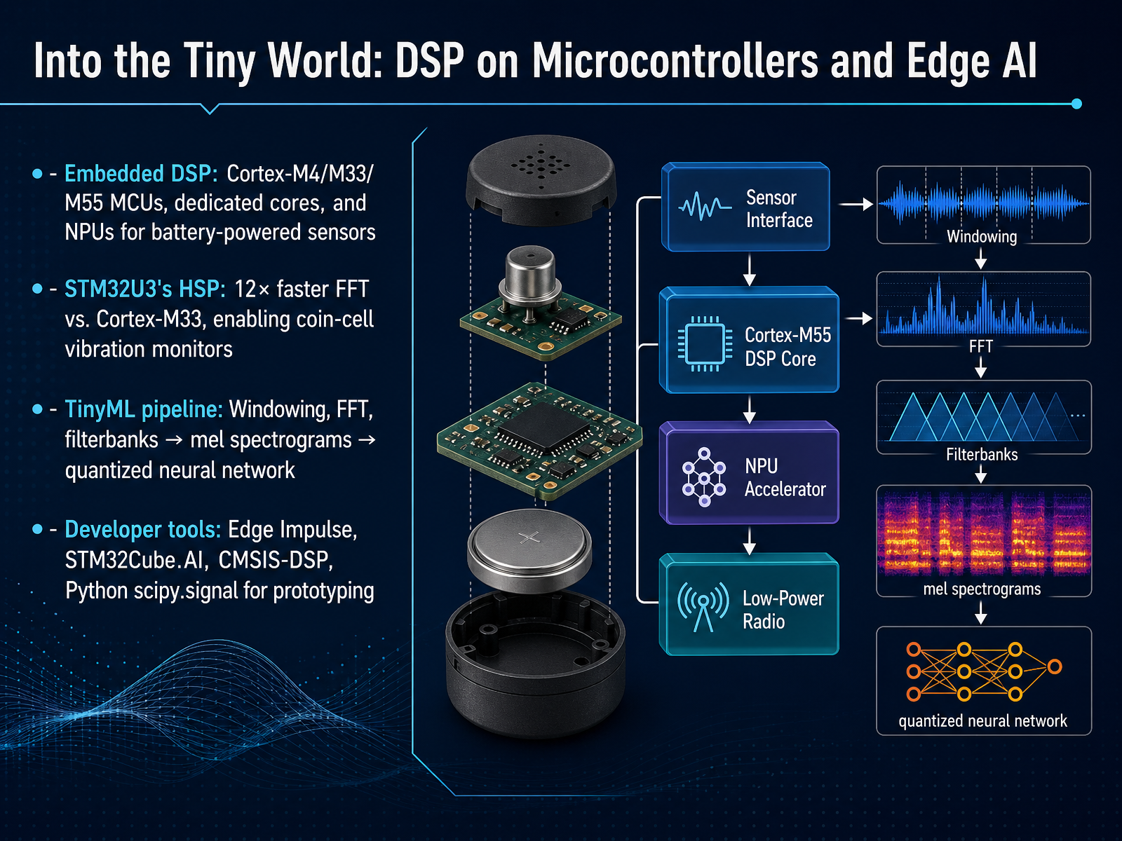
14Into the Tiny World: DSP on Microcontrollers and Edge AIWith the fundamentals of sampling, representation, and filtering behind us, let's bring digital signal processing into the tiny world of microcontrollers and edge AI. We're talking about devices so power-efficient they can run for months on a coin-cell battery. The workhorses here are embedded processors like the Cortex-M4, M33, and M55, often paired with dedicated neural processing units. A great example is the STM32U3 microcontroller, which introduces a hardware signal processor, or HSP. For a fast Fourier transform, this HSP can be twelve times faster than a standard Cortex-M33 core, making continuous vibration monitoring on a battery a reality. On the software side, a typical TinyML pipeline mirrors the theory we have covered. It starts with windowing an incoming sensor signal, computing an FFT, and passing filterbanks to create a mel spectrogram. This spectrogram is then fed into a quantized neural network running directly on the device. To build these applications, developers rely on tools like Edge Impulse for the full pipeline, STM32Cube.AI for optimized deployment, and the CMSIS-DSP library. For rapid prototyping, Python's SciPy signal module remains an indispensable companion. Let's transition now to our final slide, where we'll walk through the DSP practitioner's checklist and discuss the next steps on your learning journey.doi.org nature.com link.springer.com+22 min
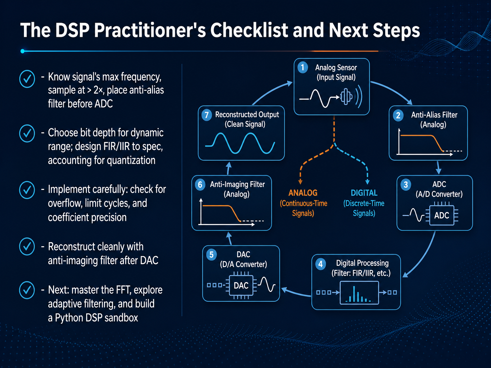
15The DSP Practitioner's Checklist and Next StepsWelcome to our final checklist, where we turn DSP theory into reliable practice. First, know your signal’s maximum frequency and sample at more than twice that rate. Always place an anti-alias filter before the ADC. This prevents high frequencies from folding back into your passband and creating permanent distortion. Next, choose your bit depth to support the needed dynamic range. Design your FIR or IIR filter to meet attenuation and phase specifications, but account for coefficient quantization from the start. When you implement, check carefully for numeric overflow, limit cycles, and coefficient precision loss—especially in fixed-point designs. Once your digital processing is complete, reconstruct the analog signal cleanly with an anti-imaging filter after the DAC. To keep growing, make the FFT your everyday tool, explore adaptive filtering, and build a Python DSP sandbox using NumPy and SciPy. These habits will make you a confident, effective practitioner. Thank you for joining this course, and good luck with your next signal.compoundlearn.ai schaumont.dyn.wpi.edu schaumont.dyn.wpi.edu+22 min

Sources consulted

Web sources consulted while building this course.