Reading Motion Graphs

This training teaches learners to interpret position, velocity, and acceleration motion graphs, building the skills to analyze and describe motion accurately.

A digital instructor presents all 14 pages. Hold “Ask” at any point and ask out loud — the answer comes from this course. No sign-up needed.

28 minFree to watchDownloads

What you’ll learn

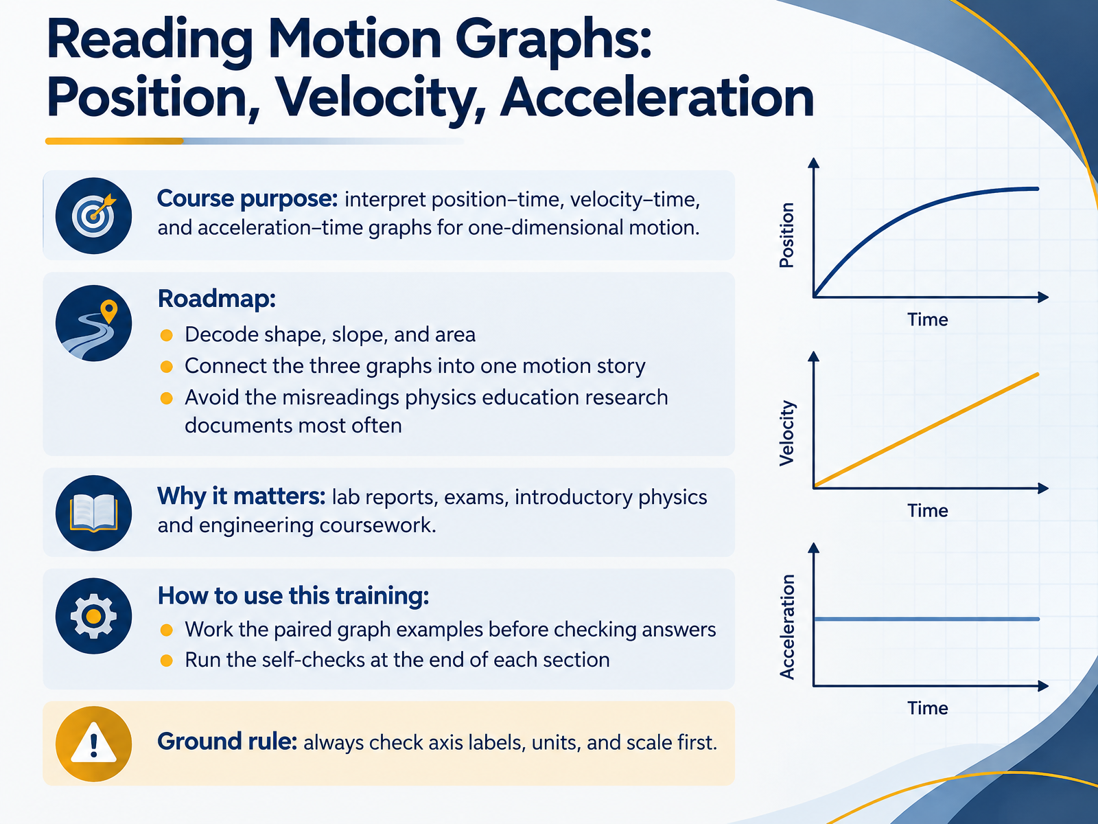
01Reading Motion Graphs: Position, Velocity, AccelerationWelcome. I'm glad you're here, because today we're going to learn to read motion graphs with confidence. Position, velocity, and acceleration graphs tell one connected story about how something moves, and by the end of this course, you'll be able to follow that story from any starting point. Here's our roadmap. First, we'll decode the three big features of any graph: its shape, its slope, and the area beneath it. Next, we'll connect the position, velocity, and acceleration graphs for a single motion, so one event becomes three consistent views. Then we'll tackle the misreadings that physics education research documents most often, like reading a graph as a picture of a path, or confusing slope with height. Why does this matter? These skills show up in lab reports, exams, and introductory physics and engineering coursework. Finally, here's your ground rule for every graph we meet. Before anything else, check the axis labels, the units, and the scale. If you predict first, then check, you'll learn faster. Coming up next, position, displacement, and sign conventions.per-central.org link.aps.org journals.aps.org+22 min
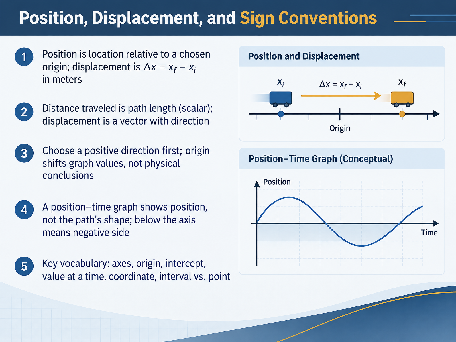
02Position, Displacement, and Sign ConventionsLet's build the foundation for reading every motion graph. Position is simply where an object is, measured from an origin you choose. Displacement is the change in position, written as delta x equals x final minus x initial, measured in meters. Distance and displacement are different. Distance is the total path length, a scalar with no direction. Displacement is a vector, so it includes direction. Before you read any graph, pick a positive direction, like right or up. The origin you choose shifts the numbers on the graph, but it does not change the physical story. Remember, a position versus time graph shows position, not the shape of the path. If the line sits below the axis, the object is on the negative side of your origin. Keep this vocabulary close: axes, origin, intercept, value at a time, coordinate, and the difference between an interval and a single point. Here is a quick check. If you walk three meters right, then three meters back, your distance is six meters, but your displacement is zero. Try predicting that on a graph before we move on. Next, we will see how slope becomes velocity when you read position versus time graphs.2 min
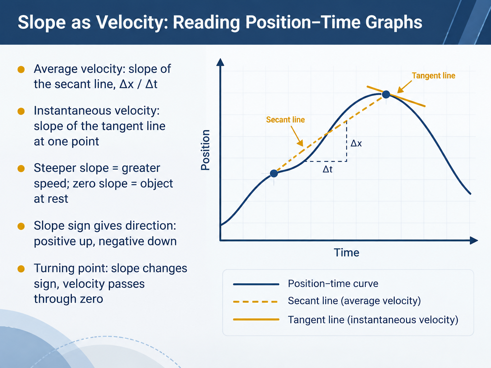
03Slope as Velocity: Reading Position–Time GraphsNow let's read motion from a position-time graph. On this graph, the vertical axis is position, and the horizontal axis is time. Here's the key idea. Slope equals velocity. To find average velocity, draw a straight line between two points, called the secant line, and divide the change in position by the change in time. For instantaneous velocity at one moment, picture the tangent line touching the curve at that single point. Its slope gives the velocity right then. Notice the patterns. A steeper slope means greater speed. A zero slope, a flat line, means the object is at rest. The sign of the slope gives direction. Positive slope means moving forward, and negative slope means moving backward. At a turning point, the slope changes sign, so velocity passes through zero. Before I reveal the next example, pause and predict this. If the line gets steeper, is the object speeding up or slowing down? Keep that question in mind. Next, let's look at a common mistake. The graph is not a picture.2 min
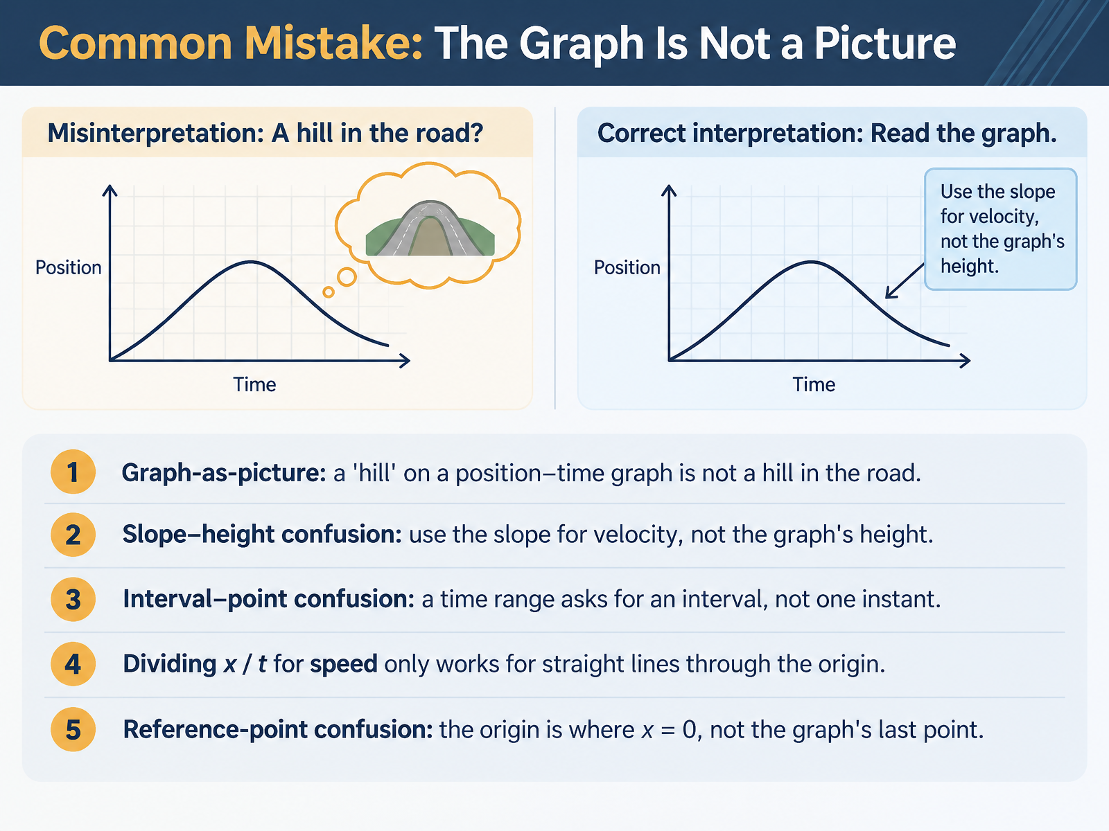
04Common Mistake: The Graph Is Not a PictureLet's clear up a mistake that trips up almost everyone at first. A position-time graph is not a picture of the motion. A hill on the graph is not a hill in the road. Picture a cyclist riding up a real hill. On a position-time graph that climb looks like a rising straight line, not a curved bump. The line is not the hill. It is a record of where the rider is over time. So why do we read it as a picture? Because our eyes treat any shape as an object. Researchers call this the graph-as-picture error, and it is completely normal. Here is the first fix. Use the slope, not the height. Slope means how steeply the line rises or falls. On a position-time graph, slope is velocity. The graph's height is position, the rider's location. So a steep line means fast, and a high line just means far from the starting point. The second fix. Match the question to the answer. If you are asked about a time range, describe that whole interval, not one instant. If you are asked about a single moment, look at that point. The third fix. Be careful with speed equals distance divided by time. That shortcut only works for straight lines through the origin, where position starts at zero. Otherwise, use the slope. And the last fix. The origin is where position equals zero, not the graph's last point. Before we move to velocity-time graphs, try predicting: if a position-time graph slopes downward, what does the velocity-time graph look like? From Position to Time, to Velocity to Time.hrcak.srce.hr researchgate.net per-central.org+22 min
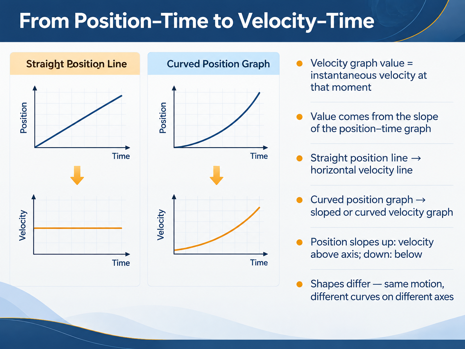
05From Position–Time to Velocity–TimeNow let's connect position and velocity graphs. On a velocity-time graph, each point tells you the instantaneous velocity, the velocity at that exact moment. That value comes from the slope of the position-time graph. Imagine walking forward at a steady pace. Your position graph is a straight line, and your velocity graph is a flat horizontal line. Now imagine slowing to a stop. Your position curve bends, so the velocity graph slopes downward. Here's a useful pattern. When the position graph slopes up, velocity sits above the axis. When position slopes down, velocity drops below the axis. The shapes differ, but they describe the same motion. Before we go on, pause and predict: if the position graph curves upward more and more steeply, what will the velocity graph look like? Next, we'll look at velocity-time graphs in detail, covering slope, direction, and the difference between speed and velocity.2 min
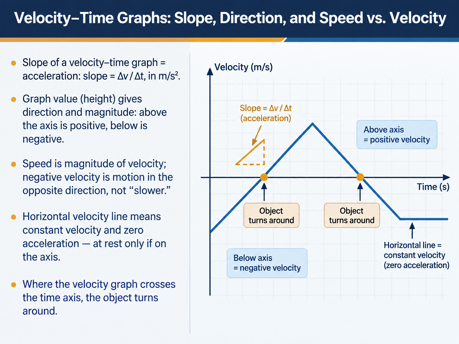
06Velocity–Time Graphs: Slope, Direction, and Speed vs. VelocityNow let's look at velocity–time graphs, where one graph answers two questions at once. The slope tells you acceleration, calculated as change in velocity divided by change in time, measured in meters per second squared. Before I go further, pause and predict: if a velocity graph is a straight horizontal line above the time axis, what is the acceleration? It's zero, because the slope is zero. The object moves at a constant velocity. But if that line sits on the axis, it's at rest. Now, the height of the graph gives direction and magnitude. Above the axis is positive velocity; below is negative. Here's a common mistake: negative velocity is not slower, it's motion in the opposite direction. Speed is the magnitude, the size, of velocity. To tell if something speeds up or slows down, compare the slope with the graph's value. Same sign means speeding up; opposite signs means slowing down. And where the graph crosses the time axis, the velocity passes through zero, and the object turns around. Next, we move to the area under a velocity–time graph, covering displacement and distance.phys.libretexts.org physicsclassroom.com savemyexams.com+22 min
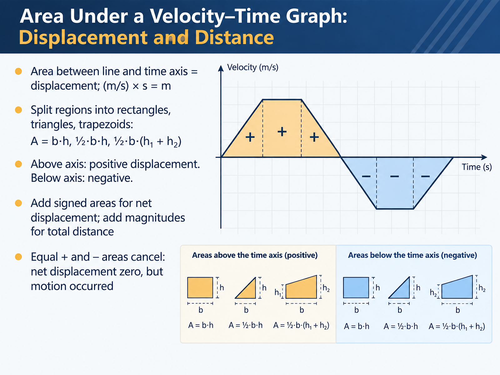
07Area Under a Velocity–Time Graph: Displacement and DistanceNow let's talk about area under a velocity-time graph. Here's the key idea. The area between the line and the time axis equals displacement. Why? Because velocity in meters per second, multiplied by time in seconds, gives you meters. A distance. To find that area, split the region into simple shapes. A rectangle uses base times height. A triangle uses one half times base times height. And a trapezoid uses one half times base times the sum of the two heights. Now watch the signs. Area above the time axis is positive displacement. Area below the axis is negative displacement. So, to find net displacement, add the signed areas. To find total distance traveled, add the magnitudes, ignoring the signs. Here's a useful example. If a positive area of ten meters is followed by a negative area of ten meters, they cancel. Net displacement is zero. But motion still occurred, so the total distance is twenty meters. Before we move on, try predicting this one. If a velocity-time graph dips below the axis for a while, what does that mean? Pause and think. It means moving backward, in the negative direction. That signed area matters. Next, we'll look at acceleration-time graphs and the slope of velocity.2 min
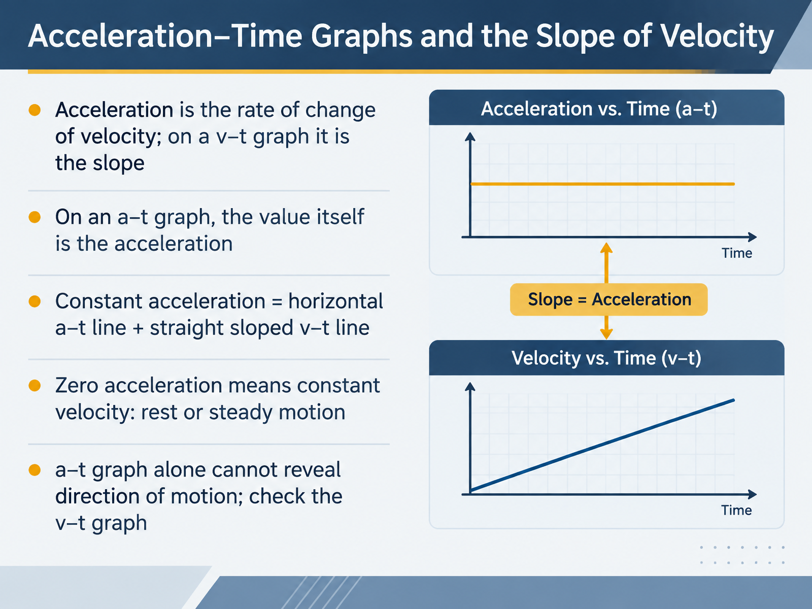
08Acceleration–Time Graphs and the Slope of VelocityNow let's look at the acceleration-time graph, or a-t graph. Acceleration is the rate of change of velocity. On a velocity-time graph, acceleration is the slope, calculated as change in velocity divided by change in time. But on an acceleration-time graph, the value itself is the acceleration. Here is a simple pattern to remember. Constant acceleration appears as a horizontal line on the a-t graph, and the matching velocity-time graph is a straight, sloped line. Zero acceleration means constant velocity, so the object is either at rest or moving steadily. Before I show the answer, pause and predict. If the a-t graph is a flat line above the time axis, what does the v-t graph look like? It is a straight line sloping upward, because velocity changes at a steady rate. One important caution: an acceleration-time graph alone cannot tell you the direction of motion. You must check the velocity-time graph for that. Remember, constant acceleration makes a horizontal a-t line, and zero acceleration means steady velocity. Next, we'll bring this together in Speeding Up, Slowing Down, and Turning Around.phys.libretexts.org physicsclassroom.com savemyexams.com+22 min
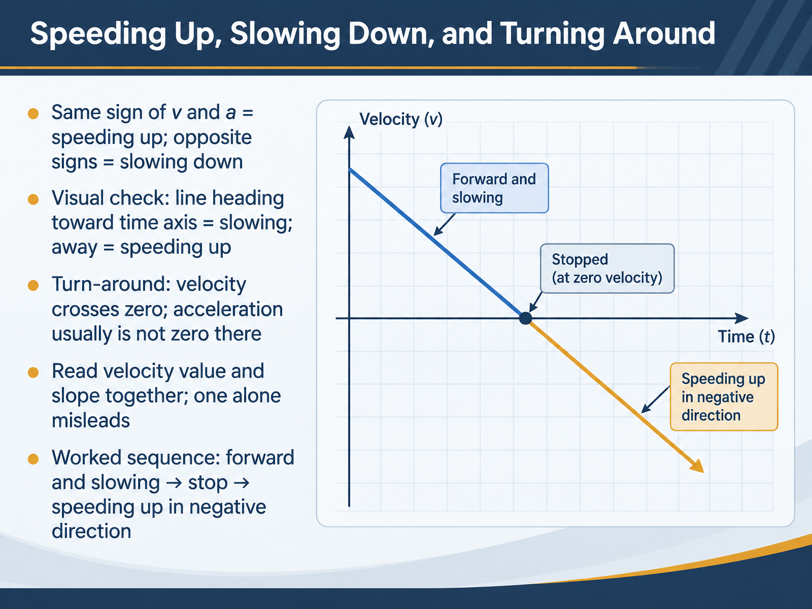
09Speeding Up, Slowing Down, and Turning AroundLet's look at how the signs of velocity and acceleration work together to tell you if something is speeding up, slowing down, or turning around. Here is the key rule. When velocity and acceleration have the same sign, the object is speeding up. When they have opposite signs, it is slowing down. Picture a car rolling forward while the driver gently brakes. The velocity is positive, but the acceleration points backward, so those signs are opposite. The car is slowing down. Now think about the same car pressing the gas while still moving forward. Both velocity and acceleration point ahead, so the car speeds up. Here is a quick visual check. On a velocity-time graph, if the line is heading toward the time axis, the object is slowing down. If the line is heading away from the time axis, it is speeding up. A turn-around happens where velocity crosses zero, and acceleration is usually not zero there. This is a common spot for mistakes, so take it slowly. Always read the velocity value and the slope together. One alone can mislead you. Here is a worked sequence. The object moves forward and slows down. Then it stops at velocity zero. Then it speeds up in the negative direction. Now, before I show the next graph, pause and predict. If an object is moving in the negative direction but speeding up, what signs do its velocity and acceleration have? Next, we will connect these ideas in Graph Translation: Slope Down, Area Up.openstax.org direct.physicsclassroom.com khanacademy.org+22 min
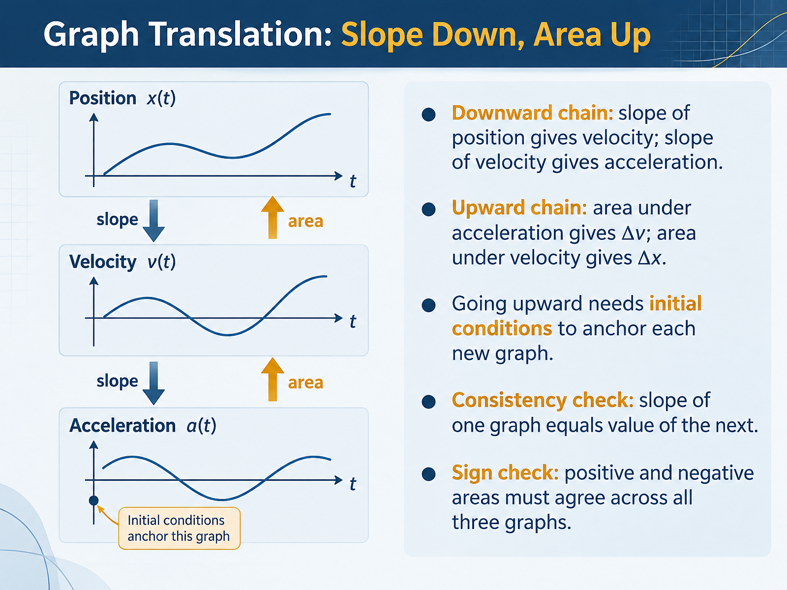
10Graph Translation: Slope Down, Area UpNow let's connect the three graphs in both directions. Going downward, the slope of the position graph gives you velocity, and the slope of the velocity graph gives you acceleration. Picture a car easing away from a stop sign: a gentle upward tilt in position means a small positive velocity. Now reverse the chain. Going upward, the area under the acceleration graph gives you the change in velocity, and the area under the velocity graph gives you the change in position, written as delta x. Here's the catch: going upward needs initial conditions. Area only tells you how much something changed, not where it started, so you need a known starting value to anchor each new graph. Keep one consistency check handy. The slope of one graph equals the value of the next. And watch the signs. Positive and negative areas must agree across all three graphs, or you have made an error somewhere. Before we move on, try predicting the next one yourself: if velocity crosses from positive to negative, what must the acceleration graph show at that moment? We will tackle common misreadings next, in Misreadings That Persist: A Diagnosis Checklist.2 min
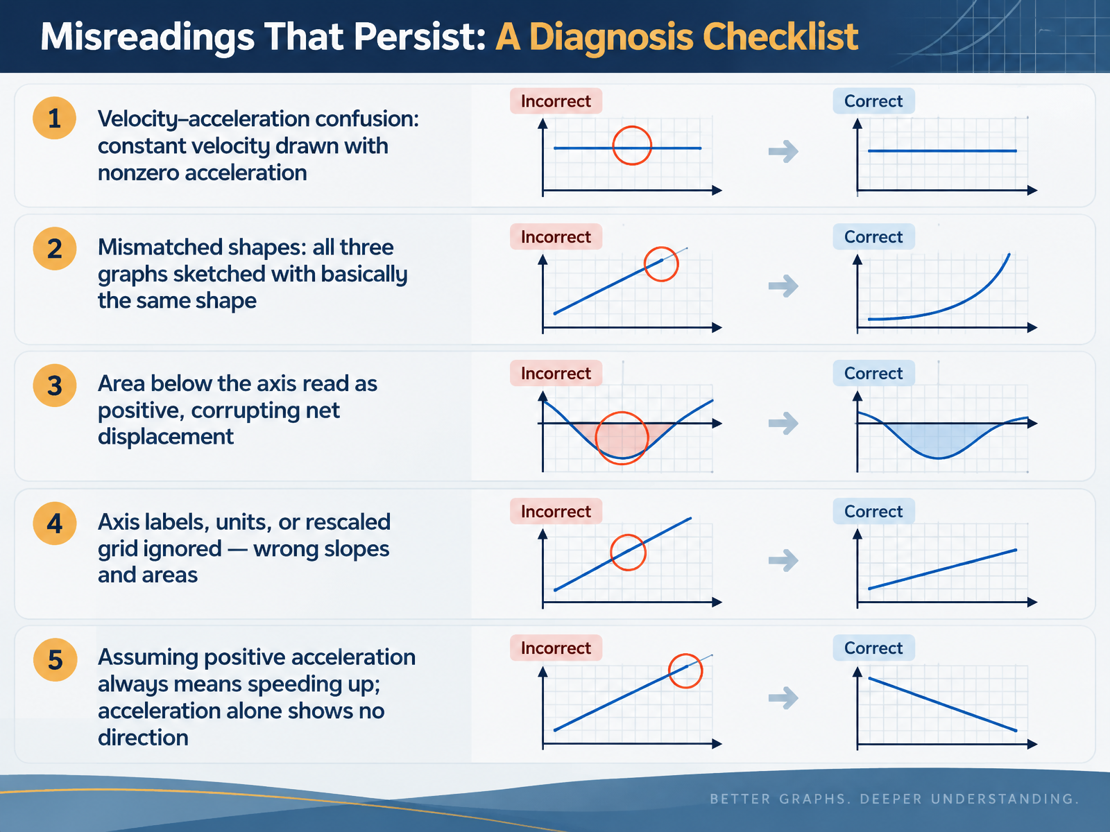
11Misreadings That Persist: A Diagnosis ChecklistLet's look at the misreadings that tend to stick around. This is your diagnosis checklist. First, velocity and acceleration get confused. A car cruising at a steady velocity is often given a nonzero acceleration graph, even though constant velocity means zero acceleration. Second, mismatched shapes. Students sketch position, velocity, and acceleration graphs that all look basically the same. The same motion needs graphs of very different shapes. Third, area below the time axis gets read as positive. That corrupts net displacement, because negative area means motion in the opposite direction. Fourth, axis labels, units, or a rescaled grid get ignored, so slopes and areas come out wrong. Fifth, assuming positive acceleration always means speeding up. Acceleration alone shows no direction; you need velocity too. Notice a theme? These errors come from treating graphs as pictures. So before you trust any reading, pause and check: what are my axes, what does the slope mean, and what does the area mean? Next, let's practice with motion sensors and graph matching.per-central.org link.aps.org journals.aps.org+22 min
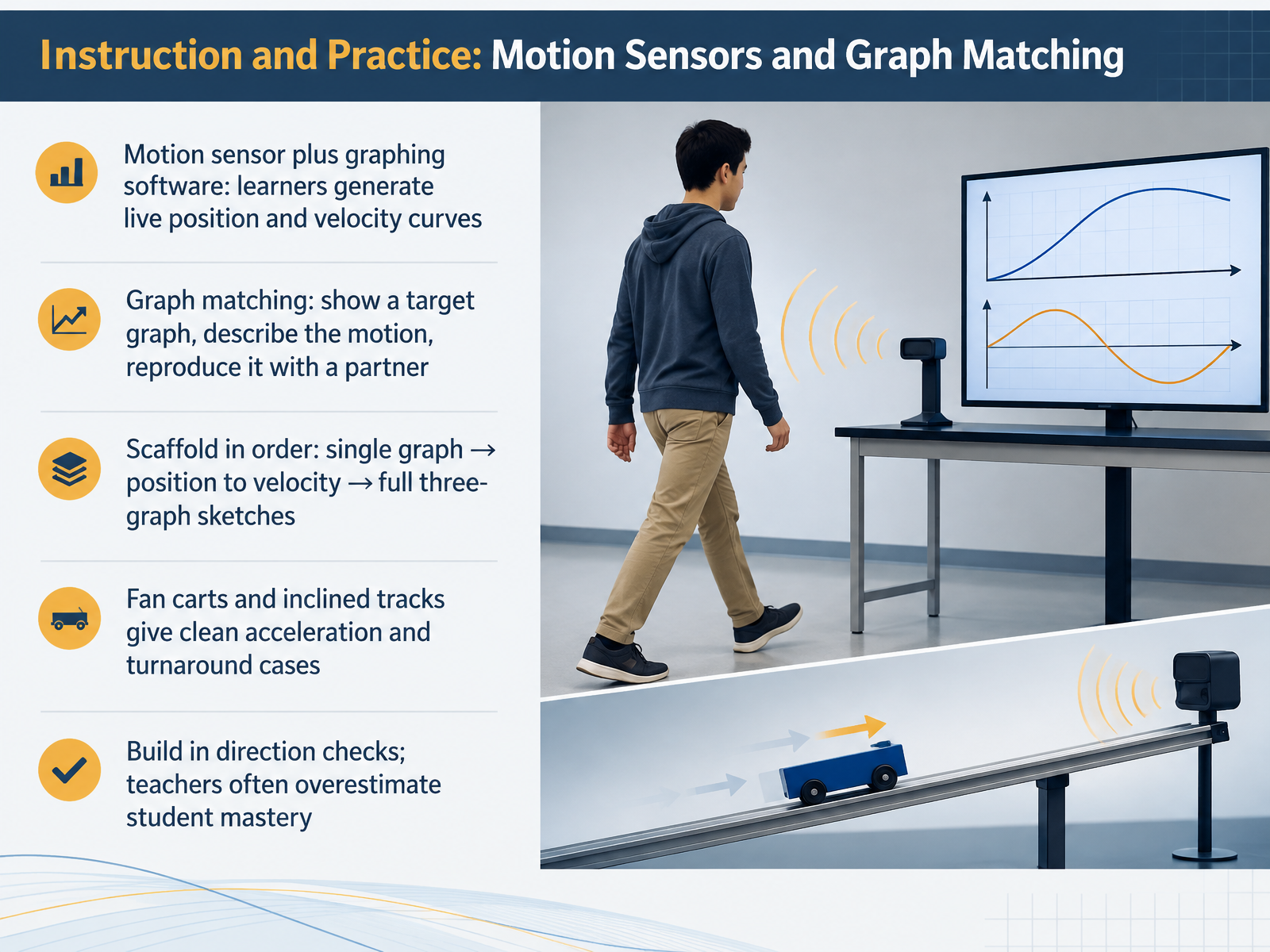
12Instruction and Practice: Motion Sensors and Graph MatchingNow let's put those reading skills into practice with motion sensors and graph matching. A motion sensor connected to graphing software lets you create live position and velocity curves in real time. You walk, you pause, you turn around, and the graph responds instantly. That immediate feedback is powerful, because you see the link between your motion and the shape of the line. Graph matching works like this. The software shows a target graph. You and a partner describe the motion it represents, then try to reproduce it. The sensor draws your actual curve right on top, so you can compare. Start simple, with a single graph. Then move from position to velocity. Finally, sketch all three graphs: position, velocity, and acceleration. Fan carts and inclined tracks are great for this, because they produce clean acceleration and nice turnaround cases. Before you reveal the answer, pause and predict what the graph will look like. One tip for teachers. Build in direction checks along the way. It's easy to overestimate how well students read these graphs, so quick check-ins catch confusion early. Next, we'll move into guided practice with slope, area, and sign in mixed graph sets.2 min
13Guided Practice: Slope, Area, and Sign in Mixed Graph SetsLet us put those tools to work with some guided practice on mixed graph sets. Practice one gives you a position graph. Look for the flat intervals, where the object is at rest. On a position graph, slope means velocity, so the steepest segment shows the fastest motion. Where the slope changes sign, the direction changes, and the height itself tells you the position value. Practice two moves to a velocity graph. Here, area matters. Area above the axis counts as positive, area below as negative. Add the signed areas to get net displacement. Add the absolute areas to get total distance. They differ whenever the object reverses. Practice three asks you to reason from an acceleration graph with three linear segments. Is the object speeding up or slowing down? Compare the sign of acceleration with the sign of velocity. Same sign means speeding up. Opposite signs mean slowing down. Practice four is a translation task. You will sketch velocity and acceleration from a described motion. Before you reveal each answer, pause and predict what the graph should show. Then check your labels, your chosen strategy of slope, area, or value, and whether your signs make sense. A good habit is to redraw the second graph and compare. Mistakes here are normal, and each one sharpens your reading. In the next slide, we will close with your action plan for continued practice.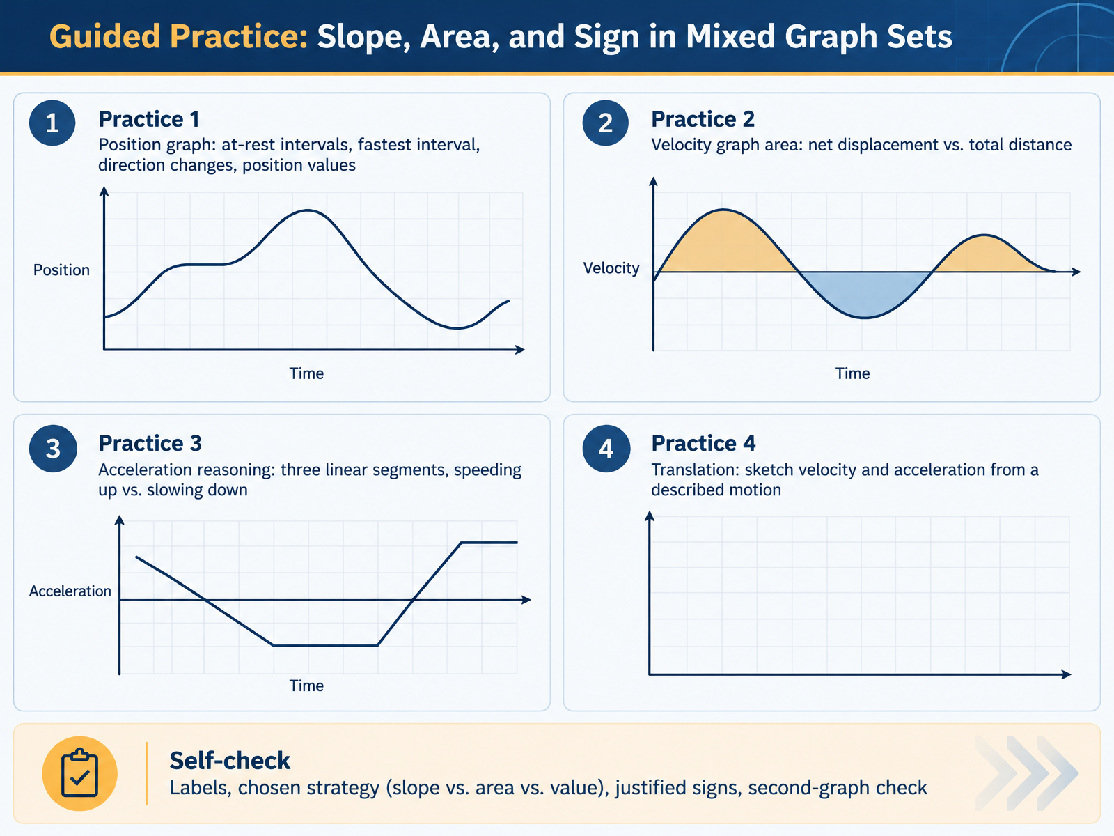2 min
14Your Action Plan: Next Steps After This TrainingYou made it, and here is how to keep this skill sharp. Four rules cover everything we practiced. Slope down, area up, the sign carries direction, and always check consistency between graphs. Turn those four words into a habit. If you are a student, redo one mixed practice set from memory, then apply your graph reading to a real lab report or problem set. For educators, run a short diagnostic on velocity and acceleration direction, since that is where confusion tends to hide, and add one graph-matching activity per unit. If you are an adult learner, master the sign conventions and physical meaning first, before chasing symbols. To go deeper, try Test of Understanding Graphs in Kinematics items, motion sensors, and constant-acceleration labs. Thank you for sticking with this training. Reading graphs is a skill you build with practice, not a talent you are born with. So pick one action, try it this week, and expect a few stumbles along the way. You are closer than you think.per-central.org link.aps.org journals.aps.org+21 min

Take the deck with you

Download this course as a file — free, no sign-up needed.

PDF handoutEvery slide page, ready to print or share.15 pages · 3.4 MBDownload
Narrated PowerPointThe deck that presents itself — every slide carries the digital human's narration video.15 pages · 15.8 MBDownload
PowerPoint slidesThe full deck as a .pptx — open it in PowerPoint, Keynote, or Google Slides.15 pages · 3.3 MBDownload

Free to use in your own training — please keep the PersonWise credit page at the end.

Have your own deck? Turn it into a course

Sources consulted

Web sources consulted while building this course.