How Operating Systems Run Programs

Name: How Operating Systems Run Programs
Availability: InStock

This training explains how operating systems manage and execute programs, covering key processes like memory allocation and CPU scheduling.

My workspace30 minFree to watch

What you’ll learn

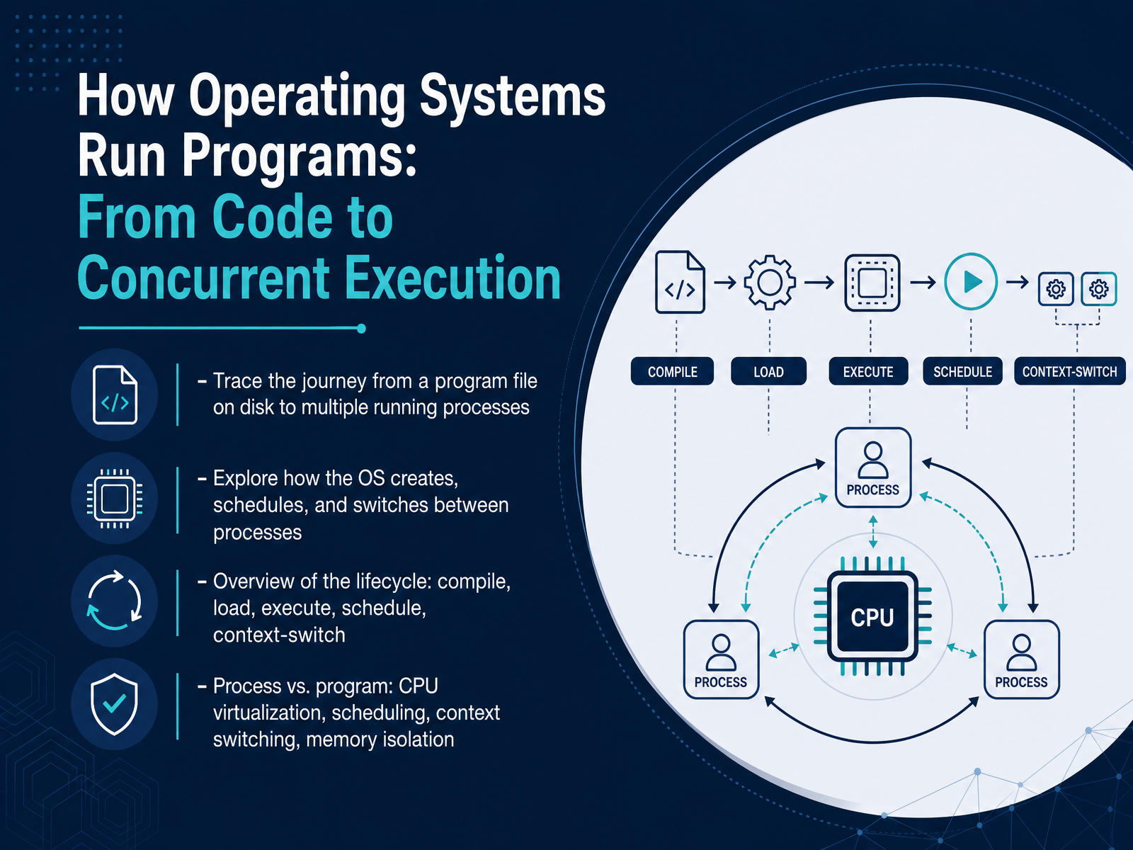
01How Operating Systems Run Programs: From Code to Concurrent ExecutionWelcome. In this course, we are going to trace exactly how an operating system takes a program file sitting on disk and turns it into multiple running processes. Our goal is to reveal the systematic choreography that makes concurrent execution possible. We will follow the complete lifecycle, from compilation through loading, execution, scheduling, and context switching. Along the way, we will clarify the essential distinction between a program and a process, and examine the mechanisms that enable CPU virtualization, scheduling decisions, context saving and restoration, and memory isolation. By the end, you will see process coordination not as a mystery, but as a predictable, step-by-step routine the kernel follows every time. Next, we begin by deconstructing a program, from binary file to address space.1 min
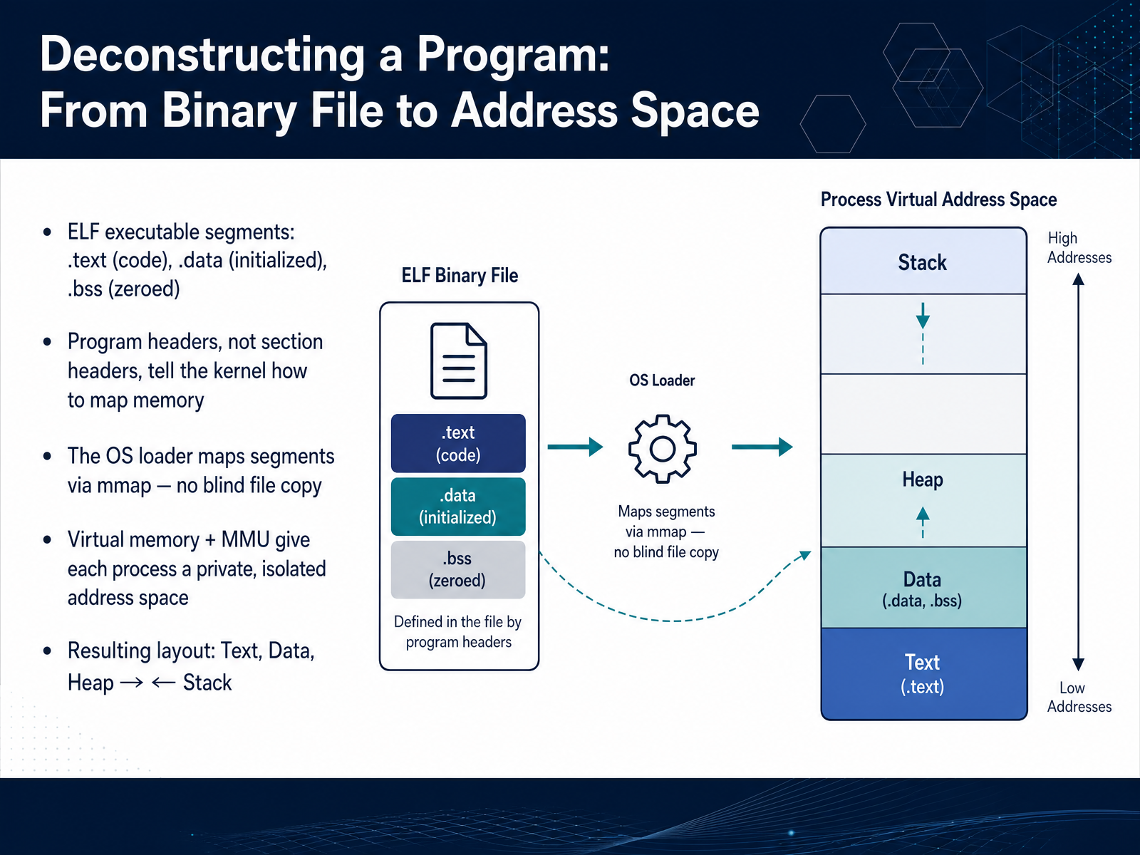
02Deconstructing a Program: From Binary File to Address SpaceNow let's look inside the executable file itself and see how the operating system transforms it into a running process. A compiled program on disk is organized as an ELF executable with distinct segments. The dot text segment holds the machine instructions, dot data carries initialized global variables, and dot bss reserves space for uninitialized data that the kernel zeroes out. For execution, the kernel reads the program headers, not the section headers. Those program headers describe loadable segments: their virtual addresses, sizes, permissions, and file offsets. When the loader processes these segments, it does not blindly copy the entire file into memory. Instead, it uses memory mapping through mmap to create virtual memory areas backed by the executable file. For the dot bss segment, the kernel maps anonymous, zero-filled pages beyond the file-backed region. The memory management unit then presents each process with a completely private, isolated address space, an illusion of owning all of memory. The final layout places the text and data segments at the bottom, the heap grows upward from the data, and the stack grows downward from a high address. This virtual address range is the foundation that the operating system builds upon before the process ever starts executing. Next, we'll explore the spark of life: how the operating system creates a process.kernel-internals.org onenoughtone.com github.com+22 min
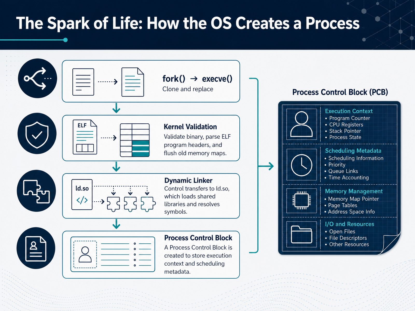
03The Spark of Life: How the OS Creates a ProcessLet’s walk through exactly how the operating system breathes life into a program and turns it into a running process. When a parent process calls fork, it creates a clone of itself. That clone then invokes execve. This is the moment the real transformation begins. The kernel opens the executable file, reads its ELF header, and validates the binary format and architecture. Then it flushes the old address space entirely. A new, blank memory layout is prepared. The kernel parses the ELF program headers and maps each loadable segment into the fresh virtual address space. It does this using private file-backed mappings, so the text segment stays read-only and executable, while data becomes writable. Critically, control does not jump directly to your program. First, the kernel maps the dynamic linker, ld.so. Then it creates a Process Control Block, or PCB, to house the execution context and scheduling metadata. Once the address space is ready, the kernel sets the instruction pointer to ld.so’s entry point and hands over control. The dynamic linker then takes over: loading shared libraries, resolving symbols, and preparing the runtime before finally jumping to your program’s start. Coming up next, we look inside the process itself at the CPU state, memory footprint, and what makes up that kernel-side tracking structure.kernel-internals.org onenoughtone.com github.com+22 min
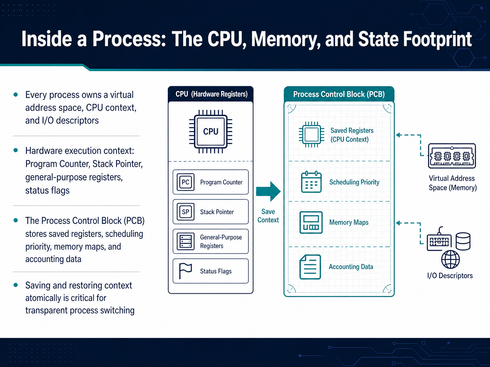
04Inside a Process: The CPU, Memory, and State FootprintNow let's open up a process and see what it actually contains. Every process owns three fundamental resources: a virtual address space for its code and data, a set of CPU register values we call the hardware execution context, and a table of I/O descriptors for open files and devices. The hardware execution context is the precise snapshot of the CPU while the process runs — the program counter pointing to the next instruction, the stack pointer, all general-purpose registers, and status flags. The operating system stores this entire footprint in a data structure called the Process Control Block, or PCB. In the Linux kernel, this is the task_struct — a single structure that holds the saved register state, scheduling priority, memory maps, and accounting data like CPU time used. When the kernel switches from one process to another, it must save this context and restore the next one atomically — as an uninterrupted operation. If any part of the save or restore were interleaved with other work, the process could resume with corrupted state. This atomic context switch is what makes multitasking transparent to user programs. Up next, we will see how these saved states map onto the formal lifecycle of a process in "The Rules of the Game: Process States and Lifecycle Transitions."linux-kernel-labs.github.io en.wikipedia.org github.com+22 min
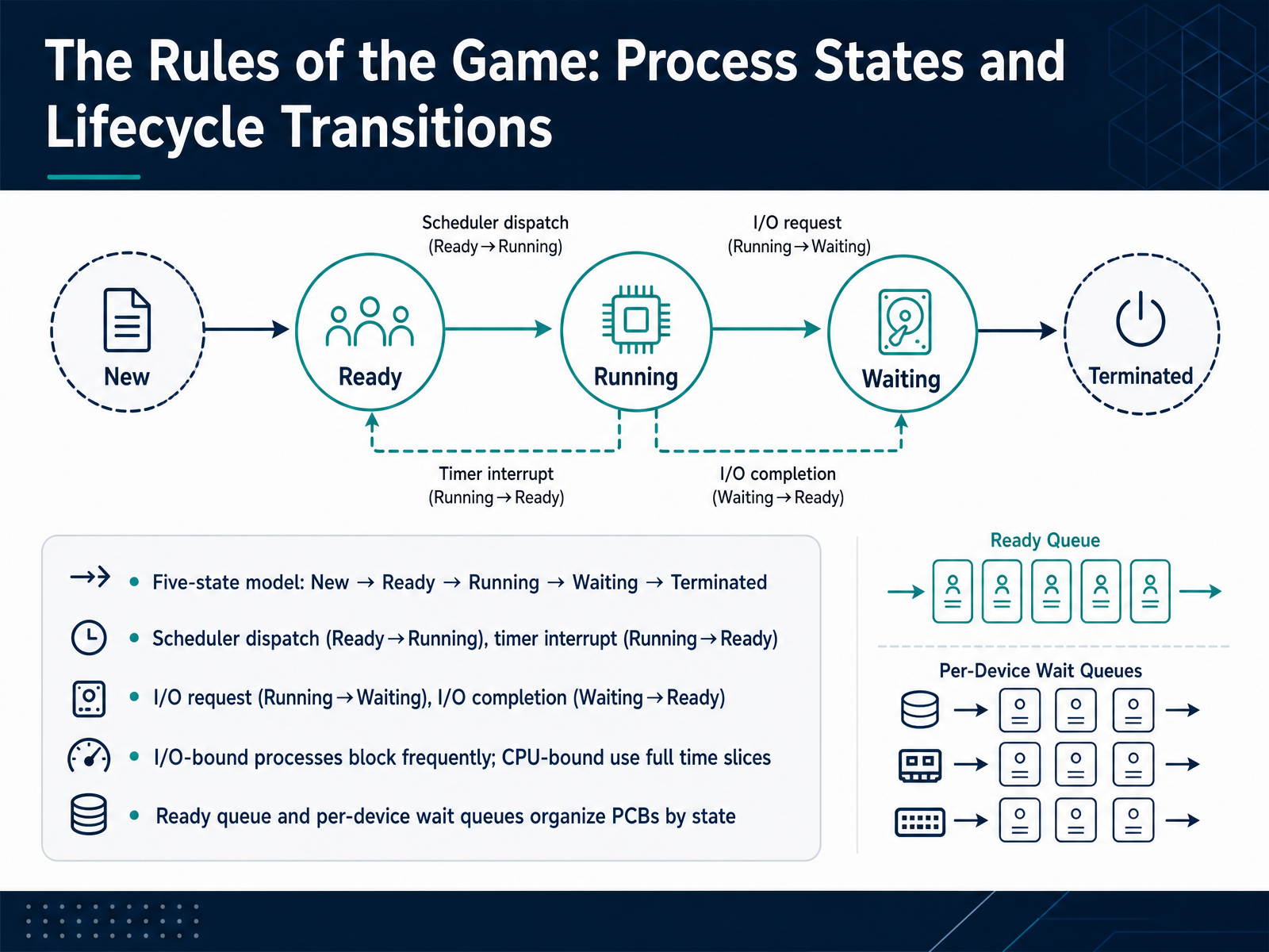
05The Rules of the Game: Process States and Lifecycle TransitionsNow let's formalize the rules that govern every process. We call this the five-state model. A process begins as New, moves to Ready when it’s prepared to run, enters Running once the scheduler dispatches it to a CPU, transitions to Waiting when it requests I/O or another event, and finally reaches Terminated when it completes or is killed. The dispatcher moves a process from Ready to Running. A timer interrupt later preempts it, moving it right back from Running to Ready so another process can use the CPU. When the Running process issues an I/O request, it blocks and moves to Waiting. Once that I/O completes, an interrupt moves it back to Ready. I/O-bound processes spend most of their time in the Waiting state, while CPU-bound processes consume full time slices in Running. The system tracks all this using queues. The Ready queue holds PCBs for processes that are Ready, and per-device Wait queues hold PCBs for processes blocked on specific I/O devices. These queues are just linked lists of process control blocks, systematically reorganized as state transitions occur. Next we’ll step inside the dispatcher and see exactly how context switching mechanics work.linux-kernel-labs.github.io en.wikipedia.org github.com+22 min
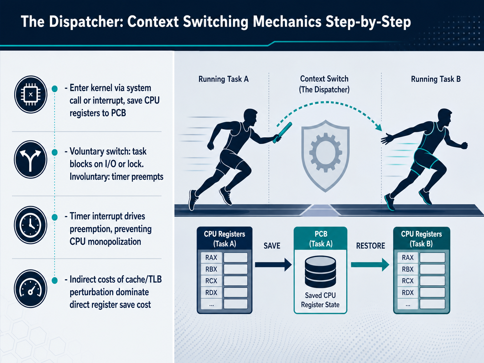
06The Dispatcher: Context Switching Mechanics Step-by-StepNow let's walk through the dispatcher's mechanics, step by step. Everything starts by entering the kernel. A system call or a hardware interrupt forces the CPU into kernel mode, and the first thing that happens is the current CPU registers are saved into the running process's Process Control Block. This snapshot is essential for a clean resume later. From here, the switch can be voluntary or involuntary. A voluntary switch occurs when the task blocks itself, for example, waiting for disk I/O or a kernel lock. The task calls the scheduler directly because it has nothing to do. An involuntary switch, on the other hand, is driven by a timer interrupt. The timer fires when a process has used its allocated time slice, setting a reschedule flag. This mechanism is the backbone of preemption. It prevents any single compute-bound process from monopolizing the CPU, ensuring the system remains responsive. While we often focus on the cost of saving registers, the real performance hit comes from indirect costs. Switching memory mappings forces the CPU to invalidate cached address translations and flush the TLB. This cold-cache and TLB perturbation dominates the overhead, far outweighing the simple register save operation. Next, we will move into the core topic of scheduling itself with an introduction to scheduling goals, metrics, and process profiles.kernel-internals.org users.ece.cmu.edu pdos.csail.mit.edu+22 min
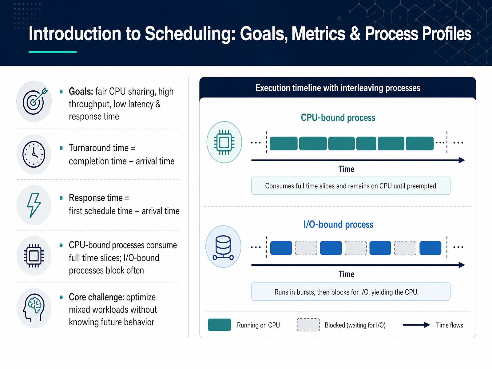
07Introduction to Scheduling: Goals, Metrics & Process ProfilesNow let's talk about what the scheduler is actually trying to achieve. The operating system has four main goals when managing the CPU. First, fairness: every process should get its share of processor time. Second, high throughput: we want to complete as many jobs as possible over a given period. Third, low latency, which means minimizing the total time a process spends in the system. And fourth, low response time: minimizing the delay between a process becoming ready and its first execution. These goals often conflict, which is why scheduling is a balancing act. We measure success with two key metrics. Turnaround time is the completion time minus the arrival time. It tells us how long a user waited for a full result. Response time is the first schedule time minus the arrival time, which tracks how quickly the system starts reacting to a request. Different processes stress these metrics differently. CPU-bound processes use their entire time slice without stopping. I/O-bound processes, on the other hand, block frequently to wait for disk or network operations. The core challenge of scheduling is optimizing for mixed workloads of both types without knowing their future behavior. 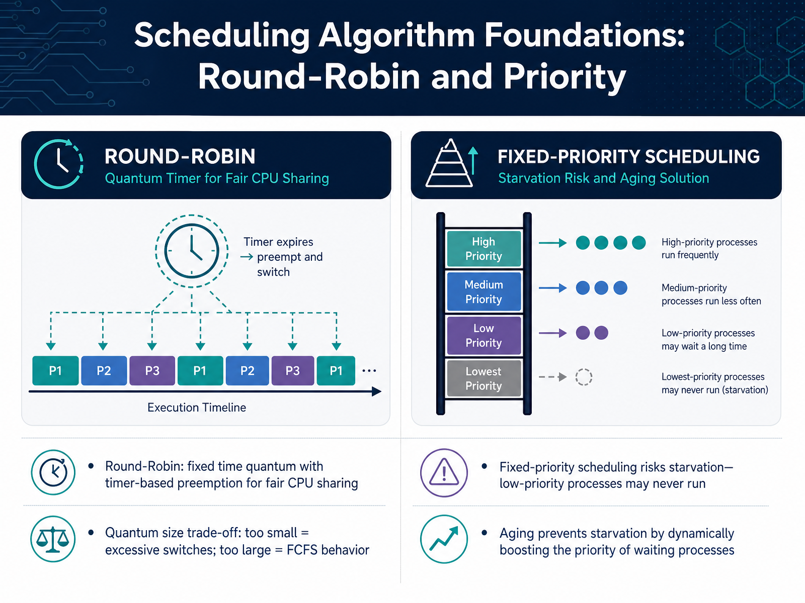Next, we will look at our first practical algorithm: round-robin and priority scheduling.2 min
08Scheduling Algorithm Foundations: Round-Robin and PriorityNow let's examine two fundamental scheduling algorithms: round-robin and priority-based scheduling. Round-robin operates on a fixed time quantum. When a process runs, the kernel sets a timer. If the process exceeds its quantum, the timer interrupt fires, forcing a context switch. This gives each ready process a fair share of the CPU in a cyclic order. The duration of the quantum matters. Set it too small, and the system spends too much time switching contexts instead of doing useful work. Set it too large, and round-robin degenerates into first-come, first-served behavior, hurting responsiveness. Priority scheduling introduces a hierarchy. A high-priority process always runs before a low-priority one. However, strict fixed-priority scheduling risks starvation. A continuous stream of high-priority work can prevent low-priority processes from ever getting the CPU. The solution is a technique called aging. The operating system dynamically increases the priority of a process the longer it waits in the ready queue. This guarantee ensures every process eventually receives service. 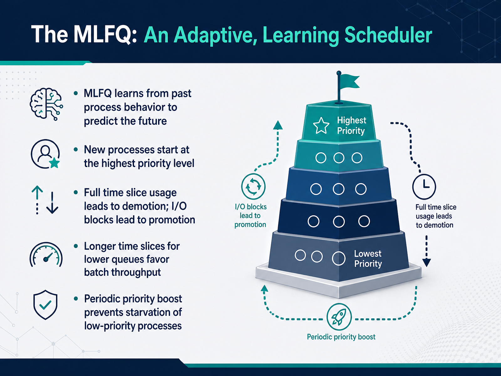Next, we integrate these ideas into a self-adjusting design: the multi-level feedback queue, or M L F Q, an adaptive learning scheduler.2 min
09The MLFQ: An Adaptive, Learning SchedulerNow let's look at how an operating system can schedule processes more adaptively. The multilevel feedback queue, or MLFQ, is a scheduler that learns from past process behavior to predict how a process will act in the future. A new process joins the highest-priority queue. If it uses its entire time slice, we interpret that as compute-intensive behavior, and the scheduler demotes it to a lower priority level. If it blocks for I/O before its slice ends, that indicates interactive behavior, and the OS promotes it or keeps it at a higher level. The lower queues receive longer time slices, which favors batch throughput for CPU-bound workloads. To prevent indefinite starvation of low-priority processes, the MLFQ applies a periodic priority boost, moving every process up to the top queue temporarily. This systematic, rule-based design creates a fair and efficient choreography, adapting as process behavior changes over time. 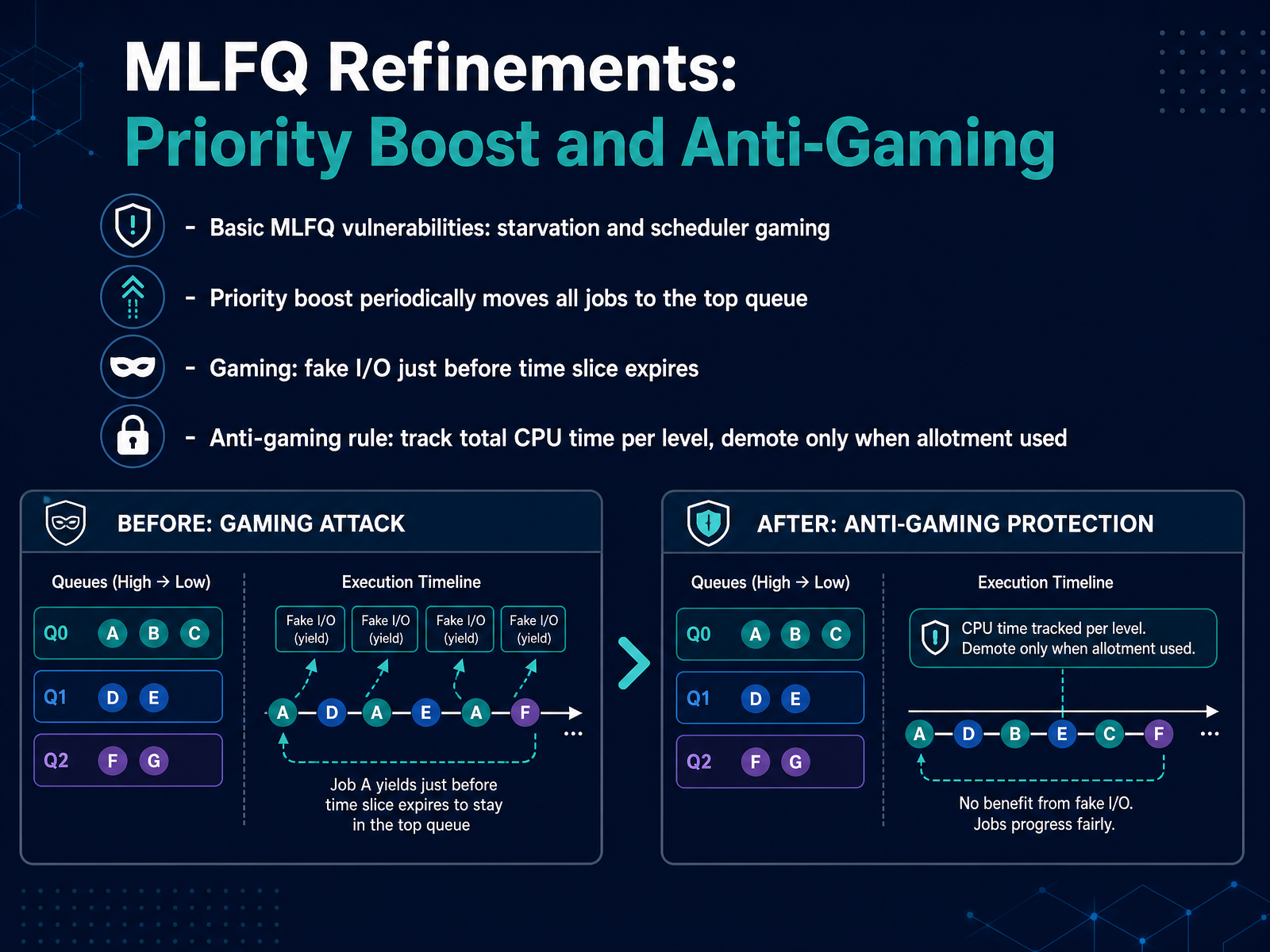Next, we will explore two critical refinements: the priority boost in more detail and mechanisms that prevent gaming the scheduler.2 min
10MLFQ Refinements: Priority Boost and Anti-GamingNow, let's address the practical problems that arise in a basic multi-level feedback queue. The design we've discussed so far is vulnerable to two specific issues: starvation and scheduler gaming. Starvation happens when short, interactive jobs constantly arrive and monopolize the top queues, leaving longer, CPU-bound jobs stuck at the bottom indefinitely. Scheduler gaming is a deliberate behavior where a process tries to trick the scheduler by, for example, performing a fake I/O operation just before its time slice expires. This makes the process appear interactive, resetting its priority and allowing it to unfairly remain in a high-priority queue. To solve starvation, we introduce a priority boost. Periodically, the operating system moves all jobs back to the highest-priority queue. This simple rule ensures that even the longest-running processes get a fresh chance to execute and prevents permanent neglect. To counter gaming, we refine the demotion rule. Instead of demoting a process every time it uses up a time slice, the scheduler tracks the total CPU time a process consumes at its current priority level. The process is demoted only when it exhausts its entire allocation for that level. A quick burst of I/O right before the time slice ends no longer resets its standing, because the scheduler looks at the accumulated runtime, not the last fraction of a second. This pair of refinements makes the multi-level feedback queue practical and robust. 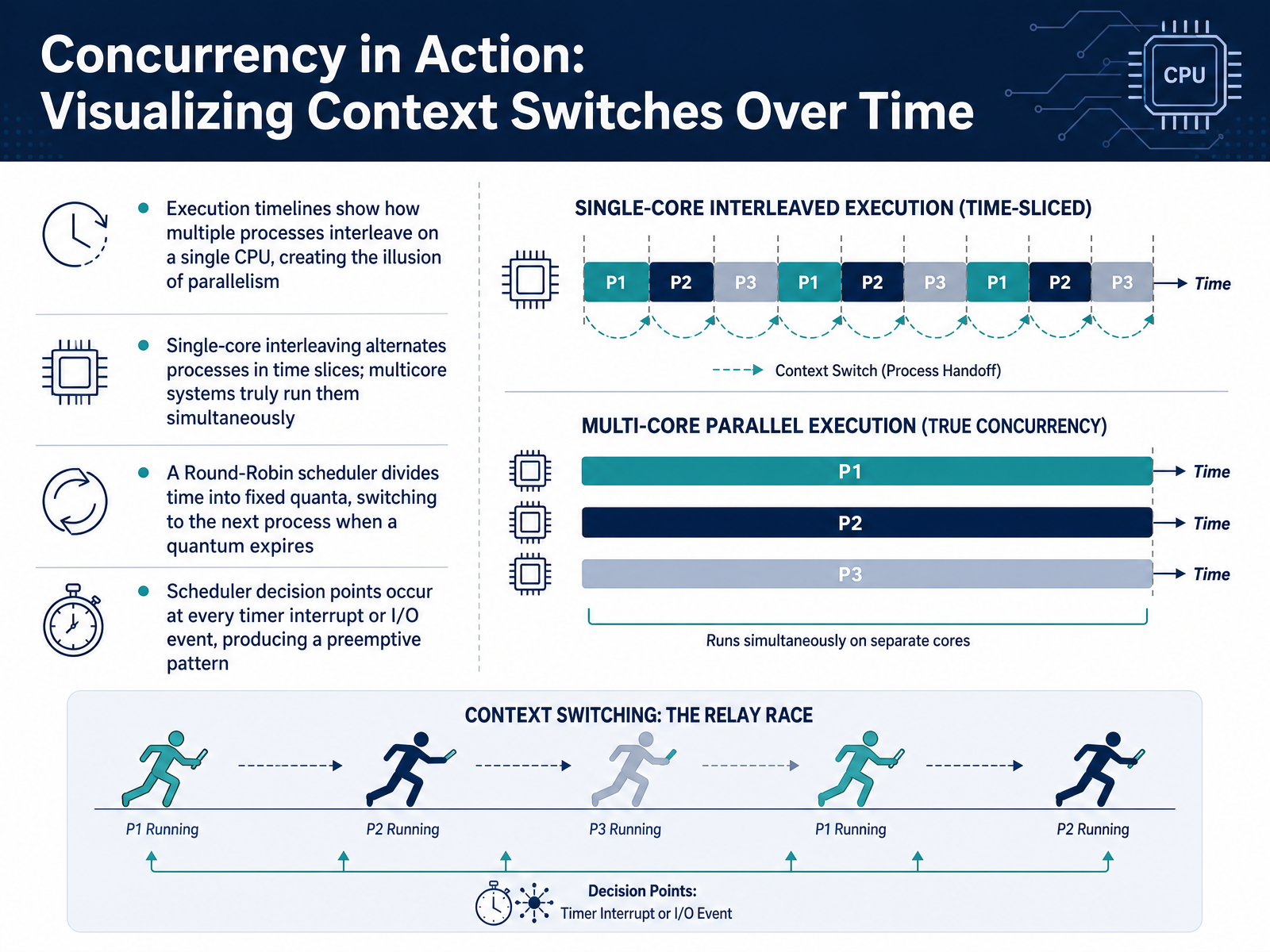Next, we will visualize these mechanics with a concrete timeline in 'Concurrency in Action: Visualizing Context Switches Over Time'.2 min
11Concurrency in Action: Visualizing Context Switches Over TimeNow let's visualize concurrency in action by looking at context switches over time. On a single CPU core, processes don't actually run at the same time. Instead, the operating system interleaves them in short bursts, creating the illusion of parallelism. With multiple cores, true simultaneous execution becomes possible. A common approach for single-core systems is Round Robin scheduling. The scheduler divides time into fixed slices called quanta. When one process exhausts its quantum, the scheduler saves its state and switches to the next ready process. This decision happens at every timer interrupt, and also when a process requests input or output, producing a preemptive pattern. The result is a timeline where multiple processes alternate in predictable, systematic order. Up next, we'll examine scheduling artifacts like starvation, priority inversion, and latency.github.com cpu-scheduling-visualizer-ribhav.vercel.app github.com+21 min
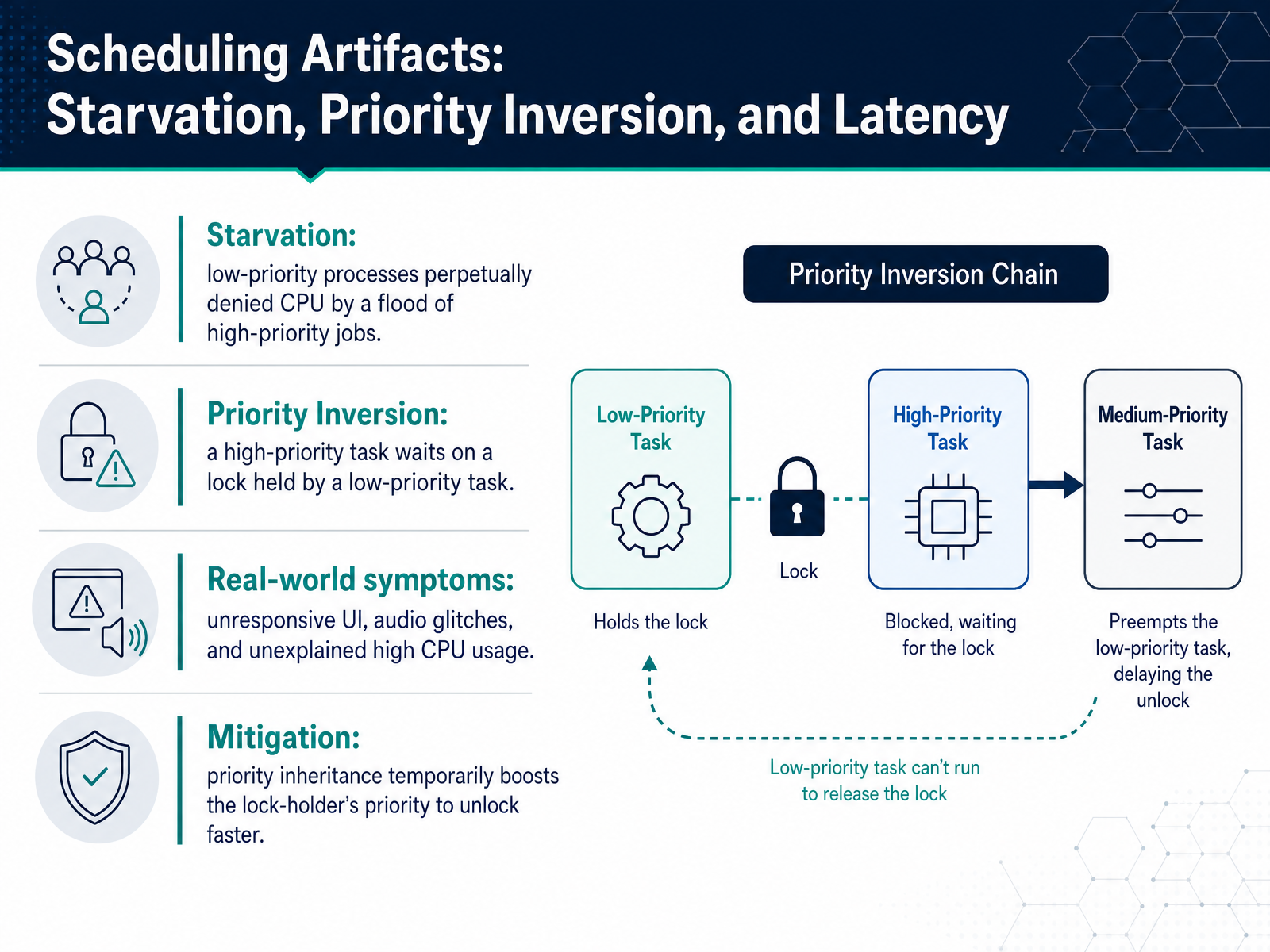
12Scheduling Artifacts: Starvation, Priority Inversion, and LatencyMoving from ideal scheduling to real-world scheduling artifacts, we encounter three terms that describe when things go wrong: starvation, priority inversion, and latency. Starvation occurs when a low-priority process is perpetually denied CPU time because a continuous flood of high-priority jobs keeps arriving. The scheduler never picks the low-priority task, so it makes no progress. Priority inversion is a more subtle problem. Imagine a high-priority task that needs a lock currently held by a low-priority task. The high-priority task must wait, but a medium-priority task, which does not need that lock, can run and effectively block the high-priority task indefinitely. This inverts the intended priority order. These are not just theoretical concerns. They manifest as unresponsive user interfaces, audio glitches, and unexplained high CPU usage in production systems. A common mitigation is priority inheritance. When a high-priority task blocks on a lock held by a low-priority task, the system temporarily boosts the lock holder's priority to that of the waiting task. This allows the low-priority task to run, release the lock quickly, and then return to its original priority, resolving the inversion. 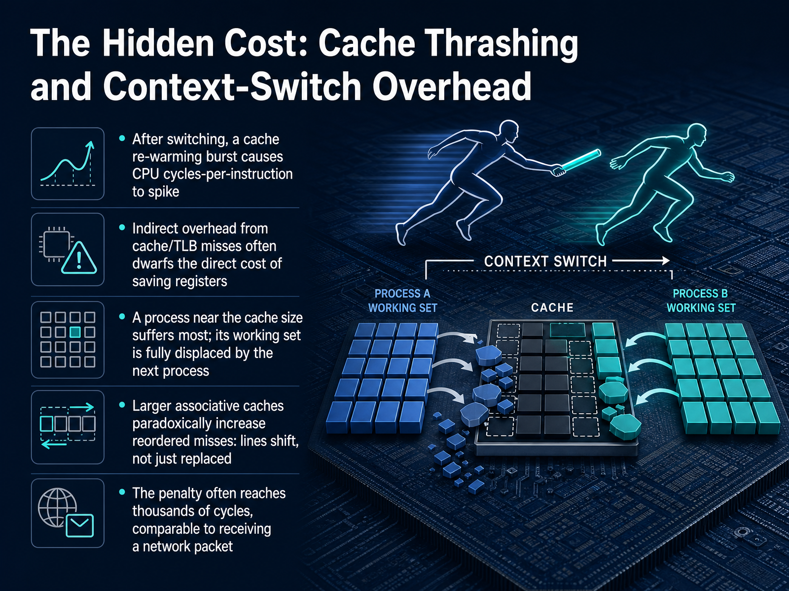Next, we examine the hidden cost of these frequent context switches: cache thrashing and context-switch overhead.2 min
13The Hidden Cost: Cache Thrashing and Context-Switch OverheadAfter a context switch, the real penalty often hits when the newly scheduled process starts running. Its working set is no longer in the cache, so the CPU goes through a cache re-warming burst. During this phase, cycles per instruction spike sharply because nearly every memory access misses and must wait on main memory. The thousands of cycles lost here can easily dwarf the direct cost of saving registers. A process whose working set is close to the cache size suffers the most. In that case, the intervening process fully displaces its data, forcing a complete reload. There is an additional subtlety with larger, more associative caches. Instead of simply replacing lines, the interfering process can reorder them, moving useful data closer to the least recently used position. These reorder misses still force eviction before the original process returns, and the penalty often reaches thousands of cycles. To put that in perspective, it is comparable to the latency of receiving a network packet. 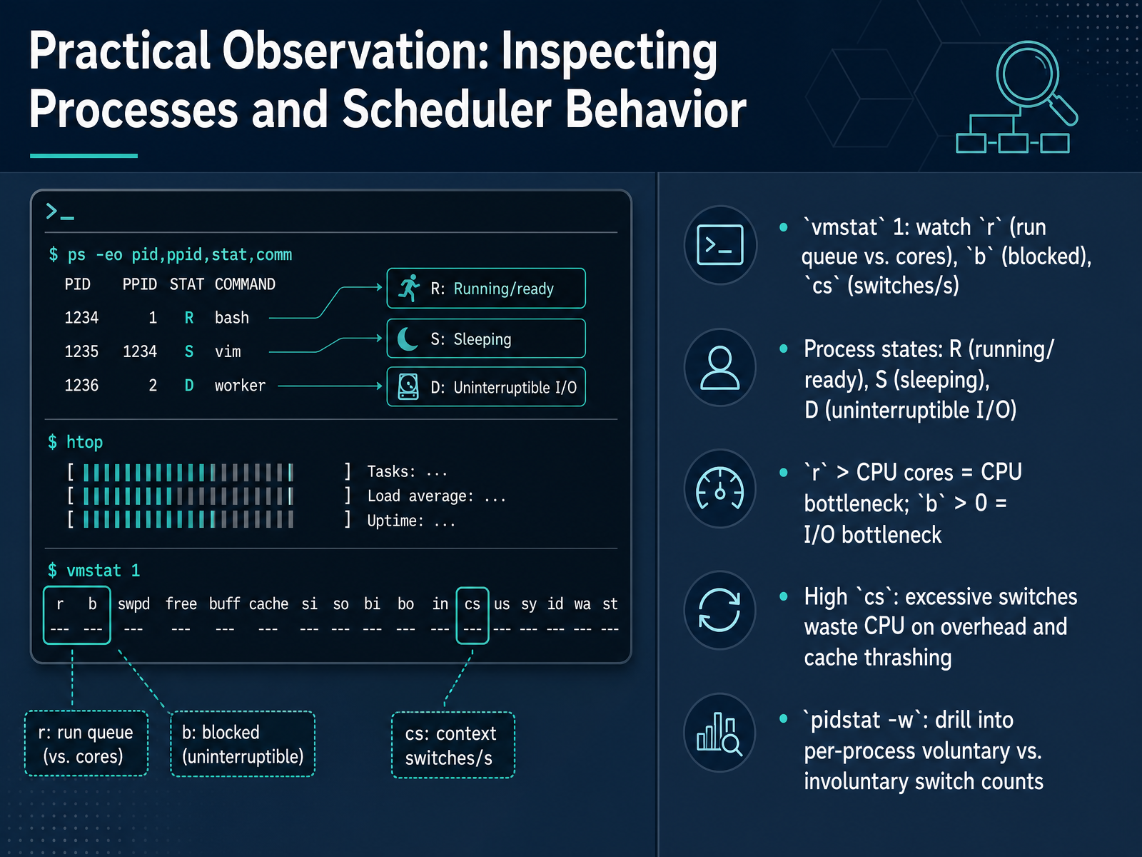Next, we turn to a practical observation: inspecting processes and scheduler behavior.1 min
14Practical Observation: Inspecting Processes and Scheduler BehaviorNow let's move from theory to practice by observing these behaviors with common command line tools. The vmstat command with an interval of one second gives us a real-time dashboard. Pay special attention to the r column, which shows the number of processes in the run queue, and b, which counts processes blocked in uninterruptible I/O. If the value in r consistently exceeds your CPU core count, you have identified a CPU bottleneck. If b stays above zero, the bottleneck is likely I/O. The cs column reports context switches per second. A sudden, dramatic spike in this number often means the system is wasting CPU cycles on overhead and cache thrashing. To understand which processes are responsible, we can drill deeper using pidstat minus w. This tool splits context switches into voluntary switches, where a process gives up the CPU willingly, and involuntary switches, where the process is preempted. High involuntary counts usually point to CPU pressure, while high voluntary counts often indicate lock contention or I/O waits. 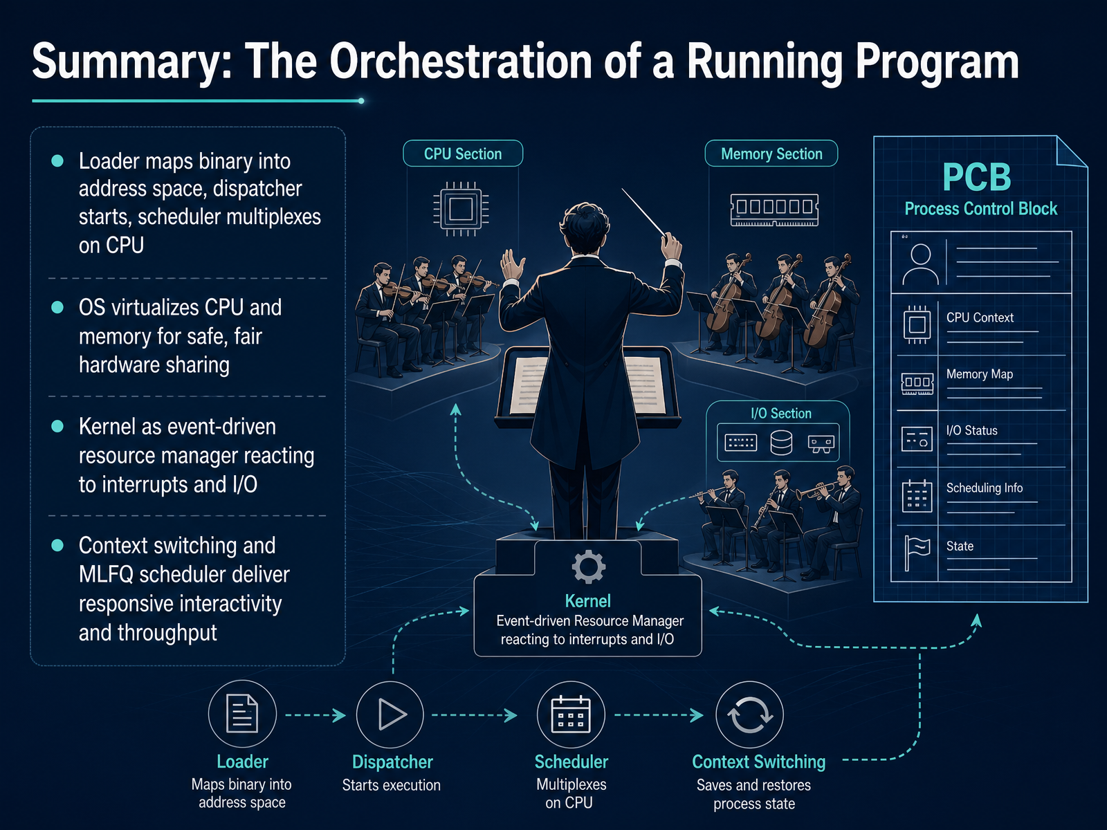Now let's wrap everything up with a final summary of how a program is orchestrated into a running process.2 min
15Summary: The Orchestration of a Running ProgramLet's bring together everything we've covered about how an operating system runs a program. The loader maps the binary into the process's address space. The dispatcher hands control to the first instruction. Then the scheduler takes over, multiplexing the CPU across all ready processes to create the illusion of simultaneous execution. The OS achieves this by virtualizing two key resources: the CPU and memory. This abstraction allows each program to behave as if it owns the hardware while the kernel enforces safe, fair sharing. At its core, the kernel functions as an event-driven resource manager. It remains idle until pulled into action by interrupts, system calls, or I/O completions. When an interrupt fires, the hardware saves a minimal context and vectors into the kernel handler. The context switch routine then saves the remaining registers of the current process and loads the state of the next one. This mechanism, combined with the MLFQ scheduler that adjusts priorities based on observed behavior, is what delivers the responsive interactivity and throughput we rely on. Thank you for completing this module. With these fundamentals, you now have a solid framework for understanding how your code actually gets executed and managed by the system.2 min

Sources consulted

Web sources consulted while building this course.